What Chromatograms Can Teach Us About Our Analytes

Gas chromatography (GC) is among the richest data-producing techniques in analytical chemistry. A chromatogram can provide a wealth of information about an individual analyte in a sample, about the sample itself, and about how well the instrument is performing. Traditional isothermal chromatograms provide useful information about the thermodynamics and kinetics of the analyte-stationary phase interactions and whether these are changing over time. They also provide measures of instrument performance through theoretical plate and tailing factor calculations. Many of these determinations are automatically performed by today’s data systems, but they trace their origins to calculations and simplifications that were done in days when chromatograms were printed on rolls of paper and calculations were done with slide rules. We will see how our data systems both assist and hinder in obtaining maximum information from chromatograms.

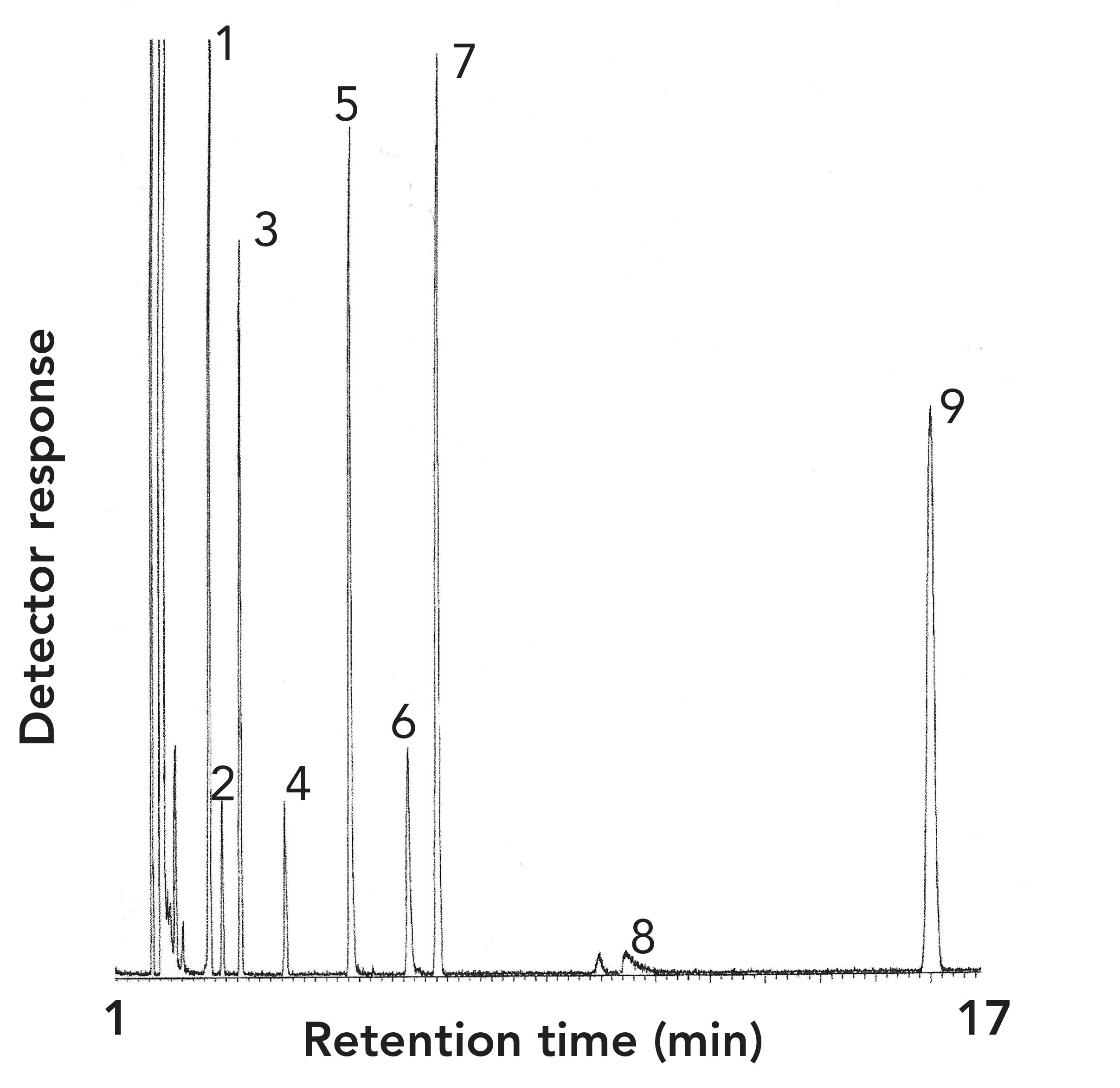
The fundamental data produced by a gas chromatography (GC) experiment is a plot of detector signal vs. time, called a chromatogram. A typical chromatogram comprised of a mixture of several common solvents is seen in Figure 1. The figure caption includes the experimental information that should be provided along with any chromatogram, including the instrument it was obtained with, carrier gas, the inlet and detector conditions, injection technique, column dimensions, stationary phase, and temperature conditions. Identities of as many of the peaks as possible should also be provided.

FIGURE 1: Isothermal chromatogram of a solvent mixture injected manually on a GC– MS system. Injection volume: 1 mL; carrier gas: helium; inlet: split 10:1, 250 oC.; column 5% phenyl polydimethyl siloxane, 30 m x 0.25 mm x 0.25 μm; Isothermal run at 40 oC. Transfer line: 280 oC. Detector: MSD, 70 ev, full scan 40–200 amu. Analytes (1 mg/mL each): 1: cyclohexane, 2: 3-methyl pentane, 3: hexane, 4: methyl cyclohexane, 5: benzene, 6: 2-pentanone, 7: heptane, 8: pyridine, 9: octane. Solvent: pentane.

In the early days of GC, most of the traditional data values, such as retention times, peak widths, and peak areas, were measured from the chromatogram by hand, using output from a strip chart recorder. Think of a paper electrocardiogram (EKG) strip in your doctor’s office or hospital, or the seismographs seen in movies. Strip chart recorders are often still used in applications like temperature monitoring. Retention times were calculated by hand by measuring the distance on the paper from the start of the chromatogram with a ruler (in cm) and dividing by the chart speed (in cm/min). Peak widths were determined by drawing tangent lines to the plot at the baseline and measuring the distance between them at the baseline. Peak areas were often determined by counting squares (chart recorders used rolls of graph paper) by cutting the peaks out with scissors and weighing them. Finally, the origins of the calculation of performance terms, like theoretical plate counts and tailing factors, go back to measuring the needed quantities by hand.

There are numerous calculations in chromatography that not only provide analytical performance data and figures of merit, but insight about the chemistry of the analyte and the separation as well. Our classical definition of the retention time, seen in equation 1 below, tells us that the total retention time (t_R) is the sum of the adjusted retention time (t’_R), the time spent sorbed on or in the stationary phase, plus the hold-up time (t_M), the time spent moving in the mobile phase.

t_R = t’_R + t_M [1]

The hold-up time is usually determined in a separate experiment or calculated from the column dimensions, gas flow rate, and temperature by the data system (1). For good chromatography, we often advise that t’_R should be at least two but not more than 20 times t_M.

The three most reported measures of a chromatographic peak, which are retention time, peak width, and peak area, each relate to a different and important aspect of the chemistry of the analyte. Retention time relates the thermodynamics of the intermolecular interactions between the analyte and the stationary phase. Peak width relates the kinetics of the sorption process at the stationary phase surface and the diffusion processes within the mobile and stationary phases. Finally, the peak area or height relates to the amount of analyte present. We will now discuss retention time and peak width, which relate to the thermodynamics and kinetics of the separation.

All chromatographic techniques (and extraction techniques) are dependent on the thermodynamics of the simple chemical equilibrium shown in equation 2, in which an analyte that begins completely dissolved or vaporized in a mobile phase partitions between being absorbed on, or dissolved in, a stationary phase. For extraction, a second stationary phase is usually substituted for the mobile phase, but the same principle of phase transition at a boundary applies. In a previous column, we discussed how this theory leads to the concept of selectivity which governs how the chemistry of solute-stationary phase interactions generates separation power (2).

A (mobile phase) ↔ A (stationary phase) [2]

The very familiar retention factor, k, is calculated as the ratio of the adjusted retention time and the hold-up time, as seen in equation 3.

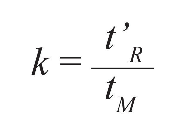
The retention factor has a deeper physical meaning, as it is also equal to the ratio of the mass of analyte sorbed in the stationary phase at a given instant to the mass of analyte vaporized in the mobile phase. This allows connection to the concentration equilibrium constant through the phase ratio, which is the ratio of the volume of the mobile phase in the column to the volume of the stationary phase, as seen in equation 4.

Classical thermodynamics that we all learned about in college chemistry classes, seen in equations 5 and 6, provide a link to the thermodynamics of the mobile phase-stationary phase transition.

∆G^o = -RTlnK [5]

∆G = ∆H = T∆S [6]

These thermodynamic quantities, calculated for many analytes on many stationary phases, provide the basis for computer simulations of GC, various retention index calculations, and discussion of column polarity.

Looking back at Figure 1, we can now draw several conclusions and inferences about the analytes present, based on intermolecular inter- actions. First, the column is considered nonpolar, with predominately dispersive interactions between the stationary phase and analytes generating retention so it follows that nonpolar analytes, such as alkanes, which also primarily interact with other molecules through dispersive interactions, would be well-retained. Also note the pattern seen in the retention times of the n-alkanes. The gap between octane and heptane is about twice as long as the gap between heptane and hexane. The gap between each successive n-alkane is about twice the time for the previous gap. This follows from the relationships in equations 3–6 and knowledge that each n-alkane differs from the next smaller n-alkane by a single -CH₂- group.

This provides a linear increase in the free energy change with the length of the carbon chain of the interaction between the analyte and the stationary phase, which translates through equations 3 and 5 as an exponential increase in the retention time. In temperature programming, which we discussed in a previous column, a linear increase in the column temperature then results in the familiar linear spacing of the homologues (3). Retention time can therefore be really thought of as a measure of the energy of intermolecular interaction between the analyte and the stationary phase. Differences in the energy generate differences in retention time and separation.

Looking at the more polar analytes in the mixture, we see that they are not strongly retained on this column, even at the relatively low temperature of 40 ^oC, which is well below all their normal boiling points and, in the higher than atmospheric pressure environment of the column, their boiling points would be further elevated. For retention times longer than the gas hold-up time to occur at all, there must be some level of intermolecular interaction between these analytes and the stationary phase. The simple isothermal chromatogram shown in Figure 1 also provides several useful clues about the performance of the column and the overall instrument, including the common calculations of theoretical plates and tailing factor.

Theoretical plate calculations, using the common expressions shown in equation 7 provide a straightforward means for evaluating overall instrument and column performance.

Peak width either at baseline or half height is the raw data point used in these calculations and this is an example of a kinetic measurement. It is well-known that as a large population of analyte molecules traverses a column, they will spread out in a generally random distribution mostly through diffusion in the mobile phase and a combination of diffusion and mass transfer in the stationary phase. The rate at which the resulting peak spreading occurs, and the randomness of the process generate the peak width and the symmetrical Gaussian shape that we expect.

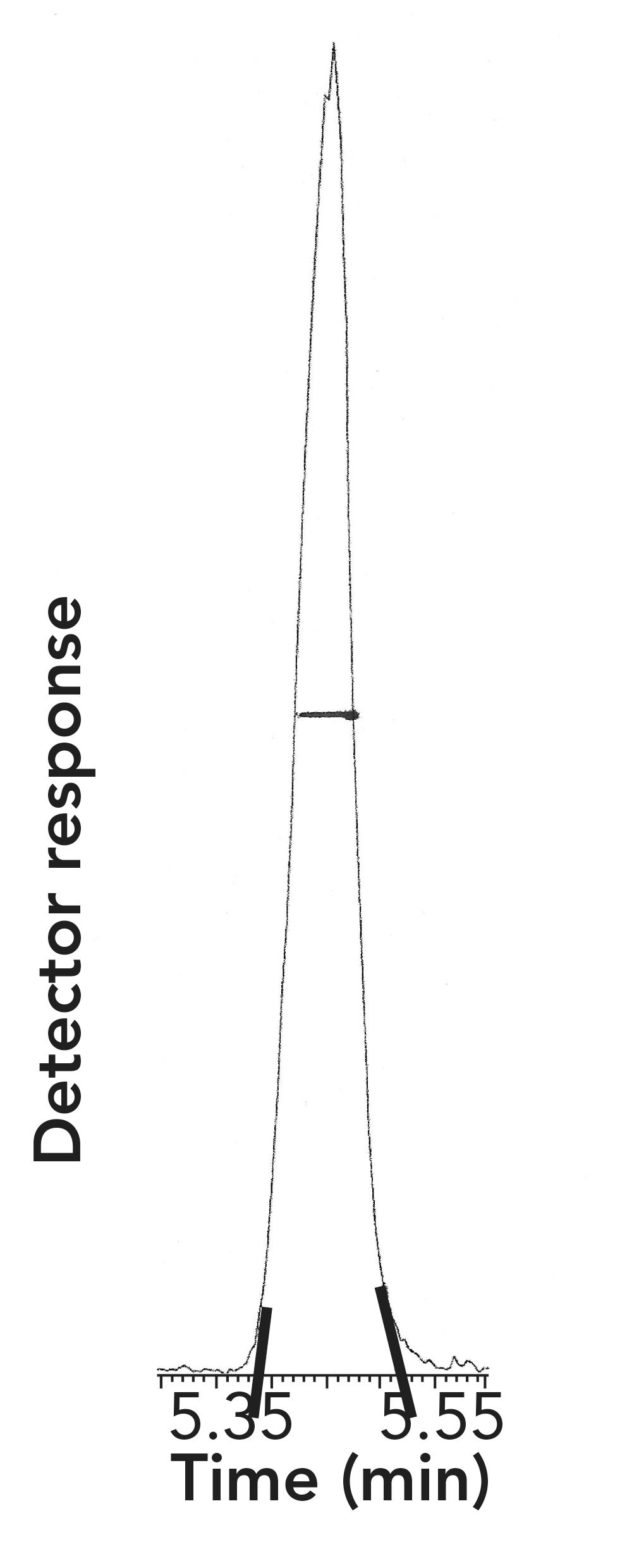
Figure 2 shows an expansion of one of the analyte peaks from Figure 1 with annotations showing the classical manual methods for determining the width at half height or baseline. An increase in peak width for all or most of the peaks in the chromatogram, perhaps following a maintenance procedure or installation of a new column is a strong indication of a problem with the installation. This is a kinetic phenomenon, usually indicating more space available for diffusion. Note the hand-drawn lines. These show the measurements that were performed to calculate N manually. If you look closely, you will see that the tangent lines, used to define the peak width at the baseline could have been drawn at several angles, possibly impacting the final calculation. When using automated calculations with a data system, beware that the data system software encounters the same problems, reminding us that many of these calculations are estimates and should be reported to only one or two significant figures.

FIGURE 2: Expanded image of the benzene peak (#5) from Figure 1 showing the measurements for calculating theoretical plates. Note the hand-drawn tangents highlighting the peak width at baseline (tangents) and half height (line).

Peak tailing (the later time side of the peak is elongated) or peak fronting (the earlier time side of the peak is elongated) are two additional kinetic phenomena that are often observed but have very different origins. Current calculations of tailing (or fronting) factors also have their roots in classical calculations done by hand.

Figure 3 shows an asymmetrical peak, with a horizontal line hand-drawn at 10% of the peak height and a vertical line from the peak maximum to the baseline. A ratio of the length of the line segment from the back of the peak to the vertical line and the segment from the front of the peak to the vertical line gives the tailing factor. A tailing factor greater than one indicates tailing and less than one indicated fronting. A tailing factor of one indicates a symmetrical peak.

FIGURE 3: Expanded image of the benzene peak (#5) from Figure 1 showing calculation of tailing factor at 10% of the peak height. Note the hand-drawn line segments highlighting the necessary measurements.

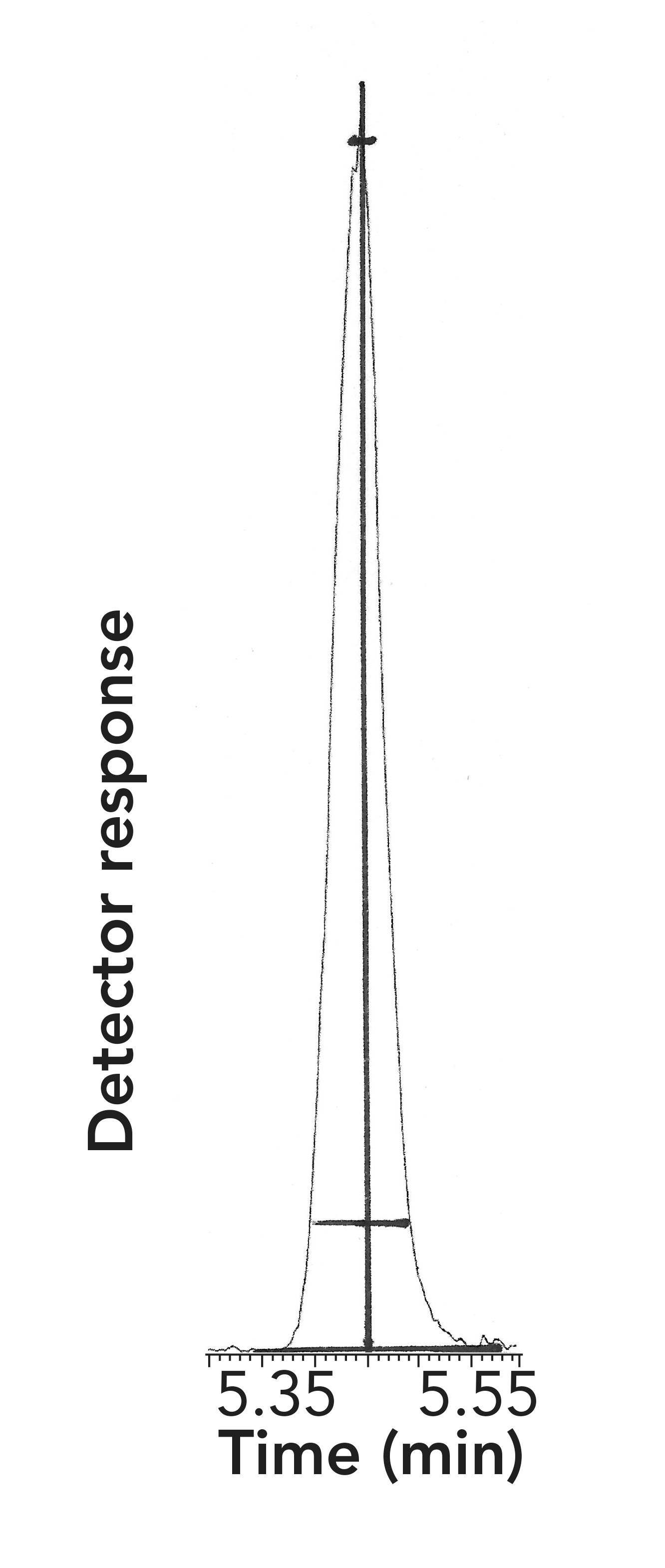
Doing these calculations by hand, at least once, provides insight in how the data system infers the beginning and end of a peak, as critical variables, when the calculation is automated. Integration parameters such as threshold, peak start and stop indicators, smoothing, and noise reduction can have an impact on how and when peak start and stop are identified and therefore on the results of calculations based on peak width and shape.

As a kinetic phenomenon, tailing of a single peak tells us that there is additional chemistry, possibly a different than expected intermolecular interaction, affecting just that one analyte. In nonpolar columns, this often occurs with polar analytes as interaction with polar surfaces within the instrument cause small additional and low-capacity retention that is superimposed on main retention mechanism in the column, thus delaying a portion of the analyte molecule population relative to the rest and generating the tail. For example, the small tailing peak for pyridine is an indication of especially strong acid-base interactions between pyridine and the column or inlet.

Fronting, seen in the peak for octane in Figure 1, has two most common causes. As seen in Figure 1, the analyte has a much higher normal boiling point than the column temperature. In this case, a portion of the analyte literally condenses on the surface of the stationary phase and is pushed ahead by the carrier gas flow (picture water in a lake or puddle on a windy day), causing it to elute early. Fronting can also be due to column overload, in which too much injected sample causes the same effect. Finally, a strong polarity mismatch between the analyte and the stationary phase can cause even low concentration analytes to exhibit fronting. This is often seen in the analysis of pyridine on nonpolar columns.

The pyridine is slightly retained by the stationary phase, but is retained by the few polar active sites on the capillary column wall. These have very low capacity so even a small sample will overload them.

Conclusion

A chromatogram can provide a wealth of information about the chemistry of the intermolecular interactions between the analytes and the stationary phase and it provides the first step in evaluating separation performance and performing instrument troubleshooting. We discussed common parameters that are often calculated automatically by today’s data systems but have their roots in hand-performed calculations that chromatographers have been practicing for decades. It is worthwhile to make printouts and perform these calculations at least once, to gain insight about the work the data system is doing, how it is doing it, and where it might make errors.

References

(1) S. McCann, H. Rana, B.A. Handzo, and N.H. Snow, LCGC North Am. 38(3), 152–158 (2020).

(2) N.H. Snow, LCGC North Am. 36(11), 806–811 (2018).

(3) N.H. Snow, LCGC North Am. 37(7), 450–456 (2019).

ABOUT THE AUTHOR

Nicholas H. Snow is the Founding Endowed Professor in the Department of Chemistry and Biochemistry at Seton Hall University, and an Adjunct Professor of Medical Science. During his 30 years as a chromatographer, he has published more than 70 refereed articles and book chapters and has given more than 200 presentations and short courses. He is interested in the fundamentals and applications of separation science, especially gas chromatography, sampling, and sample preparation for chemical analysis. His research group is very active, with ongoing projects using GC, GC–MS, two-dimensional GC, and extraction methods including headspace, liquid–liquid extraction, and solid-phase microextraction. Direct correspondence to: LCGCedit@mmhgroup.com