Pinning Down Tailing Peaks, Part II: Quantitative Measurement

In the world of practical chromatography, peak shapes only approach an ideal Gaussian statistical distribution. Solute band shapes are perturbed by extracolumn volumes, nonideal retention processes, and strong adsorptive interactions as they move from inlet to column to detector. The first installment in this series discussed some reasons for the appearance of distorted peak shapes in gas chromatography (GC) and presented various ways of expressing the degree of peak tailing (1). Beyond just cosmetic appearance, however, chromatographers have good reasons for concern over the effects of peak tailing: distorted peak shapes affect the measurement of peak height and area, and they degrade the resolution of adjacent solutes. The extent of these effects depends not only upon the degree of peak tailing but also on the size of peaks relative to the noise level and baseline drift, as well as in relation to each other. Significant peak tailing increases uncertainties due to noise and drift; even large isolated peaks can be misquantified when they tail. This "GC Connections" installment discusses the effects of tailing on the quantitative measurement of single peaks.

Of course, few peaks stand alone in complete resolution from their neighbors. The determination of the size of partially merged symmetrical peaks is a difficult task that is complicated by disparities in peak sizes as well as by peak tailing. Selective response such as that provided by diode-array detection (DAD) or mass-selective detection (MSD) can deconvolve merged peaks, but when provided with nonselective detection methods analysts must resort to baseline approximations. This will be the subject of a subsequent installment.

John V. Hinshaw

Which Peak Tailing Measurement to Use?

The previous installment (1) presented several peak tailing measurements: the ratio of peak back to front widths at a percentage of the peak height, a related pharmacopoeial measurement, the ratio of the back and front peak areas, and some statistical determinations. Back to front ratios are the simplest and most widely recognized expressions of peak asymmetry — this metric, taken at 10% of the peak height, is utilized in this installment.

For the interested reader, Ettre wrote about the origins and significance of various peak tailing measurements in LCGC in 2003 (2).

Measuring the Size of Tailing Peaks

A 2004 "GC Connections" installment (3) discussed the basics of peak detection with chromatography data systems. In that article, synthetic generated peak areas were measured as a function of the size of the peaks in relation to their minimum detectable quantities (MDQ) and the noise level for peaks with constant asymmetries of 1.5, which were intended to model an average amount of peak tailing. This month's "GC Connections" extends the measurement of peak areas across a range of peak asymmetries in another paper experiment.

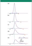
Figure 1: Effect of peak tailing on baseline allocations: (a) asymmetry = 1.1; (b) asymmetry = 1.4; (c) asymmetry = 2.0; (d) asymmetry = 2.5; and (e) asymmetry = 3.0. The green "B" symbol indicates baseline start and the orange "B" baseline stop. The baseline is drawn over the peak in blue. Inset: Peak from (e) expanded 20 times in the y-direction to show missing area in gray. The vertical dashed green line shows how the peak apex shifts as tailing changes compared to the symmetrical peak in (a).

The determination of peak starting and ending baseline points for integration and height measurements is affected by peak tailing. Figure 1 illustrates what happens when peak tailing increases with a constant baseline — no noise, no drift. In Figure 1e, an inset shows the peak magnified by 20 times in the y-direction. Peak detection found the end of the peak while a significant portion had yet to be eluted, so that a small area, filled in gray, is missing from the peak area measurement that spans the base points. Figure 2 is a graph of the measured peak area as a function of the peak asymmetry: at an asymmetry of 3.0 the measured peak area has decreased by 800 µV-s, or a little more than 5%, compared with a symmetrical peak.

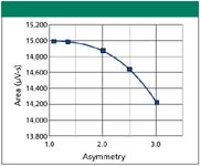
Figure 2: Effect of peak asymmetry on measured area counts for the six peaks in Figure 1.

The slight upward slope in the baseline is a minor effect compared to the loss of overall peak height as the asymmetry increases. The height of the strongly tailing peak in Figure 1e is slightly less than 50% of the height of the nontailing peak in Figure 1a. The decrease in peak height affects quantitative measurements based upon peak height, but more importantly, it reduces the ratio of the peak height to the baseline noise — a measurement related to the signal-to-noise ratio. The loss of peak height as asymmetry increases degrades the MDQ for a peak compared to the same substance if its peak shape were more symmetrical. A 50% loss in peak height translates to a 50% increase in the MDQ; this is a good reason to keep peak tailing under control.

In the case of a standalone peak on an otherwise flat baseline, the return of the second derivative to within a set threshold level is an indicator of baseline end, as shown in Figure 3. In this example, the threshold is set larger than optimum to accentuate its effect. The approach of peak derivatives toward their threshold levels on the back side of the peak is slower for all derivatives, including the first derivative (not shown), than is the initiation at the start of the peak.

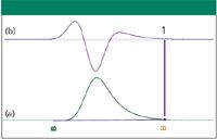
Figure 3: End-of-peak detection: (a) peak with asymmetry = 3.0 and (b) second derivative of (a). The purple band in (b) represents the threshold level below which the second derivative must return to signify the end of the baseline. Here, the second derivative returns below its threshold at point 1.

The end of the baseline is found before the peak has been completely eluted, relative to how it is found at the start of the peak, because of the peak tail. This asymmetry in the derivative values, which reflects the asymmetry of the peak itself, causes its area to be underestimated unless further processing can be performed to revise the baseline endpoint. It would seem logical to select a much lower threshold setting to move the baseline end to a later time and reduce the area measurement shortage for the peak in Figure 1e compared to the peak in Figure 1a. In fact, setting the threshold level 40 times smaller for the peak in Figure 1e does increase the measured area to 14,934 µV-s, or within 0.5% of the area of the peak in Figure 1a. The threshold choice has a strong influence when noise is present, as discussed later in this article.

There are many methods with which to determine the base points of a single standalone peak. One integrates the detector signal and compares the incremental area attributed to two or more data slices to an area threshold for peak start and stop. But in this case, the incremental areas attributed to individual data slices at the end of a tailing peak will be less than at the start and so the peak areas will again be underestimated if the threshold is too large. There are additional, more involved calculations and baseline corrections that many commercial chromatography data systems employ to help minimize the effects of peak asymmetry.

The extent of asymmetry-related effects will depend upon the data processing software, of which there are many flavors to be found in chromatography laboratories. The simple examples shown here are not intended to represent any particular data system: they are for illustrative purposes only. I found it easy to misconfigure on purpose one of the commercial systems by overriding the defaults to create a method that underestimated the areas of tailing peaks. The default settings did fairly well but the best results were obtained by using the onscreen interactive tools for configuring the system to process tailing peaks correctly. This involved setting appropriate detection thresholds and filtering parameters, and the results were quite good. In any case, chromatographers should examine baseline allocations carefully and regularly. Do not settle for default data processing settings — use the built-in tools of your data system to optimize peak detection and measurement.

Nonlinear Response

Peak tailing itself does not tend to change quickly from run to run, but it is likely to increase gradually over time as columns degrade or inlets become contaminated. Peak asymmetry also can be related strongly to the amount of injection: many compounds with tailing tendencies will exhibit much more pronounced asymmetry at low concentrations than at higher concentrations.

Regular single-level calibration of tailing peaks can provide sufficient accuracy when the sizes of tailing peaks tend not to change much from run to run, and where calibration peaks are close in size to solute peaks, because the data system's determination of the baseline points will be similar for both analyte and calibration peaks. The peak shapes of the calibrant and analyte also should follow similar trends over time as columns age. If a larger dynamic range is encountered or anticipated for a tailing peak, however, the effects of peak tailing on the baseline can contribute significantly toward response nonlinearity.

Figure 4 illustrates the responses measured with a series of increasingly large peaks with the same shape as the peak in Figure 1e, where the asymmetry equals 3.0. Again, these peaks were processed on purpose with method settings that accentuate the effects of tailing. The response (measured peak area divided by generated peak area) falls off to 87% as the relative amount drops from 100 to 1. The fraction of the total area at the end of a tailing peak that is omitted becomes smaller as peaks become larger. The peak in Figure 1e falls at the relative amount of 3.0 indicated by the arrow in Figure 4.

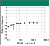
Figure 4: Measured peak response as a function of peak area. The target peaks have the same shape as the peak in Figure 1e. Peak response is expressed as the ratio of the input generated peak area to the measured peak area. The vertical arrow in this plot indicates the position of a peak the same size as the peak from Figure 1e.

Chromatographers might want to avoid injecting known tailing compounds at levels low enough to manifest significant nonlinearity. They should consider modifying sample preparation and injection techniques so that the amounts of solute on the column do not fall too low and peak tailing is curtailed. If this is not possible, then multilevel calibration using an appropriate nonlinear function might make sense in this situation. However, tailing peaks close to the noise level — or even not so close — can degrade the confidence of positive peak identification as well as yield increased uncertainty in quantitative measurement.

The Role of Noise

This discussion of the measurement of asymmetrical peaks has addressed some effects of peak tailing on peak area as either the amount of peak tailing or the area of a tailing peak change. This is all well and good, but in a real chromatograph, the level of baseline noise strongly affects area measurements as well.

Figure 5 illustrates what happens when noise is added to peaks with varying degrees of tailing. Nine repeat simulations were run on peaks with areas of 0 (blank runs), 100, 200, 500, 1000, 2000, and 5000 arbitrary units, for peaks with asymmetries of 1.1 (see Figure 1a), 2.0 (see Figure 1c), and 3.0 (see Figure 1e). The average areas and standard deviations are plotted in each part of Figure 5 as blue points with green error bars. Blank runs are represented at the far left of the plot, labeled "B" on the x-axis. As peak tailing increased, not all peaks were detected — the orange lines in Figure 5 show the percentage of trials in which the peaks were detected.

Figure 5: Measured peak areas and peak detection hit percentage as a function of input tailing peak areas at a low peak detection threshold: (a) asymmetry = 1.1; (b) asymmetry = 2.0; and (c) asymmetry = 3.0. Average peak areas are plotted in green. Error bars represent one standard deviation above and below the average area value; number of trials n = 9. Detection percentages plotted in orange are the number of times a peak was detected at each level, out of all nine trials at that level. The data point and error bars on the far left, labeled "B" on the x-axis, represent the results of running peak detection on noise only - an injection of "zero." Noise: 7.5 µV average RMS value.

Figure 5 also shows the effect of peak tailing on the peaks' minimum detectable quantities. The noise level and peak sizes were set purposely so that an amount of 200 approximates the MDQ for a symmetrical peak, where MDQ is now taken to be the peak size (area) that is twice as large as the average area of the random peaks that are detected in the presence of noise alone. The peak detection threshold was set low enough to induce detection of noise fluctuations as peaks. In Figure 5a, noise-only peak detection gave an average value and standard deviation that is the same (allowing for statistical fluctuations) as the area average and standard deviation with a peak size of 100. This indicates that the system is not capable of differentiating between purely random noise fluctuations and peaks of this size.

At a peak size of 200, the average measured value moves above the random detection level and the relative standard deviations decrease. The detection-hit percentage shows that the system has successfully found the peak in 100% of the trials at this level. As the peak size increases further, the average measured areas increase proportionately and at each level, 100% of the peaks are detected. This is good but somewhat idealized behavior, as would be expected with this kind of paper experiment using idealized peak shapes.

As peak tailing increases, however, the results change significantly and the minimum detectable quantities begin to degrade and become larger. Figure 5b shows the results of another set of simulations, this time with a peak that has asymmetry of 2.0, the peak from Figure 1c. The data are quite similar to Figure 5a at amounts greater than 1000, but under that level, peak detection becomes less reliable and the MDQ degrades a little. A measurable average response was obtained at the 200 level, but not all of the peaks were detected. Due to their reduced height and broadened profile, these asymmetrical peaks are more likely to be perturbed by the noise, and their retention times can become more widely distributed. When a detected peak's retention time falls outside the retention time identification window for the known analyte position, the peak will not be identified as the target analyte. In this manner, peak tailing will influence the confidence level of peak identification.

Figure 5c shows this effect more obviously, now with the strongly tailing peak from Figure 1e. The minimum detectable quantity clearly has increased to more than 200, and reliable peak detection no longer occurs until the amount approaches 2000. Increasing peak asymmetry from 1.1 to 3.0 has degraded the MDQ by a factor of two or more while considerably decreasing the reliability of peak detection and identification.

Conclusion

Peak tailing strongly affects the measurement of peak areas. Data system parameters should be adjusted appropriately, preferably by using the data system's built-in tools, so that peaks can be measured accurately. In the presence of normal chromatographic baseline noise, tailing peaks are more susceptible to random errors of detection and measurement than are symmetrical peaks of the same size. These errors in turn degrade minimum detectable quantities and reduce confidence in positive peak identification at low levels.

Analysts can control the effects of peak tailing by taking steps to control or eliminate conditions that lead to asymmetrical peaks. Regular monitoring of instrument and column health with check samples, increasing injected amounts of known tailing peaks, and judicious choices of data processing method parameters will help bring tailing side effects under control.

John V. Hinshaw "GC Connections" editor John V. Hinshaw is senior Research Scientist at Serveron Corp., Hillsboro, Oregon, and a member of LCGC's editorial advisory board. Direct correspondence about this column to "GC Connections," LCGC, Woodbridge Corporate Plaza, 485 Route 1 South, Building F, First Floor, Iselin, NJ 08830, e-mail lcgcedit@lcgcmag.com. For an ongoing discussion of GC issues with John Hinshaw and other chromatographers, visit the Chromatography Forum discussion group at http://www.chromforum.com.

References

(1) J.V. Hinshaw, LCGC 27(3), 232–244 (2009).

(2) L.S. Ettre, LCGC 21(1), 12 (2003).

(3) J.V. Hinshaw, LCGC 22(10), 990–997 (2004).

Erratum

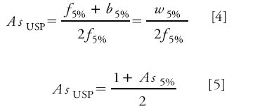
In the first installment on peak tailing (1) there are errors in equations 4 and 5. The correct equations are