Calibration Curves, Part V: Curve Weighting

This is the fifth and final installment in a series of "LC Troubleshooting" columns about various aspects of calibration of liquid chromatography (LC) methods and problems related to calibration. We have looked at questions related to whether or not the calibration curve should pass through the origin (1), how to determine method limits (2), the use of %-error plots to highlight potential problems (3), and which calibration model to use (4). This month will focus on a more specialized topic, the use of curve weighting. This also is an appropriate topic, because it addresses questions submitted by several readers asking why I didn't weight the curves in the discussion of whether or not the calibration curve passed through the origin (1).

John W. Dolan

Why Weighting?

When a least-squares linear regression is used to fit experimental data to a linear calibration curve, equal emphasis is given to the variability of data points throughout the curve. However, because the absolute variation (as opposed to %-error) is larger for higher concentrations, the data at the high end of the calibration curve tend to dominate the calculation of the linear regression. This often results in excessive error at the bottom of the curve. One way to compensate for this error and to give a better fit of the experimental data to the calibration curve is to weight the data inversely with the concentration, a process called curve weighting. The weighting of calibration curves often will lower the overall error of the method and, thus, improve the quality of the analytical results. Most LC calibration curves that span several orders of magnitude show increasing error with increasing concentration, whereas the relative error (percent relative standard deviation, %RSD) is reasonably constant. Curve weighting should be evaluated whenever the relative error is fairly constant throughout the calibration curve (5).

There also are regulatory reasons why curve weighting should be considered. The FDA's guidelines for validation of bioanalytical methods (6) contains this statement (my italics): "Standard curve fitting is determined by applying the simplest model that adequately describes the concentration–response relationship using appropriate weighting and statistical tests for goodness of fit." How are "simplest," "adequately," and "appropriate" determined? It seems to allow many interpretations, however, one key point is that weighting should be evaluated, and the evaluation of the impact of curve weighting allows for statistical tests to be applied.

Evaluation of Data

A thorough evaluation of the appropriateness of curve weighting and selection of the weighting factor is best done at the end of method development or during method validation when a sufficiently large data set is available to calculate standard deviations at each calibrator concentration. However, because most LC calibration curves exhibit similar characteristics from the standpoint of weighting, we can use a few shortcuts for the present discussion.

The first step is to determine if the standard deviation at the lower limit of the curve is significantly different from that at the upper end. This determination is based upon the F-test, which compares standard deviations for two populations. However, this test is a bit moot for the case of LC calibration curves that span two or more orders of magnitude. In almost every case, the standard deviation (or absolute error) will increase with concentration, causing the null hypothesis of the F-test to be rejected. An alternative way to come to the same conclusion is that the %RSD is fairly constant throughout the curve. We know the latter to be the common observation. For example, the FDA's guidelines for validation of bioanalytical methods (drugs in biological matrices, such as plasma) suggest that the method precision and accuracy be ≤±15% at all concentrations above the lower limit of quantification (LLOQ) and ±20% at the LLOQ. It is clear that the FDA expects the error to be approximately constant throughout the calibration curve — this is the nature of LC calibration curves. So after testing a couple of data sets to satisfy yourself, you probably can skip the F-test.

The next step is to determine the proper weighting factor for the data. The calculations are based upon a fairly complex equation that can be found in references 5 or 7. For my own satisfaction, I programmed this into an Excel spreadsheet, but by the time I entered all the formulas and debugged them so that I could get the same answers as the textbook, I had spent an entire day. A much easier approach is to use the curve weighting options that are built into most data analysis software packages. These allow you to choose a weighting factor – 1/x⁰ (no weighting), 1/x^0.5, 1/x, and 1/x² are the most useful weighting calculations. Each weighting factor will produce a weighted least squares calibration curve, which can be used to calculate the %-error (also called relative error) for each experimental value.

You can compare the effectiveness of the various weighting schemes at reducing method error by calculating the sum of the absolute values of the relative error (ΣRE). The weighting factor that gives the smallest ΣRE is the best choice. You will find that the ΣRE will drop quickly as weighting is increased, then stabilize. I suggest using the least amount of weighting that minimizes the error, as is shown in the examples in the following section. This should satisfy the FDA's "simplest model that adequately describes the concentration–response relationship using appropriate weighting" (6).

For Example

To illustrate curve weighting, I've chosen four data sets summarized in Table I. Sets 1–3 are data obtained from two different laboratories for three methods for the analysis of several drugs in plasma using LC–tandem mass spectrometry (MS-MS). In each method, two calibration curves were run, one at the beginning of the sample set and one at the end, with the data combined for calibration purposes. Internal standards were used in each case, and I have shown only the analyte/internal standard ratio in Table I. Data set 4 is a repeat of the data of Table I in the first installment of this series (1) for an externally standardized method.

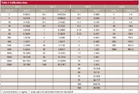
Table I: Calibration data

Let's look first in a bit more detail at data set 1, then consider the others briefly. In Figure 1, I have plotted the %-error for the data of set 1 with the various weighting schemes. It is obvious that there is a big problem at lower concentrations for the data with no weighting (open squares) and 1/x^0.5 weighting (open triangles). In fact, the %-error is so large that these weighting schemes preclude the use of the method at concentrations below 50 ng/mL. The remaining weighting schemes (solid points) look similar on this scale. Figure 2 is a plot of the same data as in Figure 1, but includes only 1/x (solid circles), 1/x² (open squares), and 1/x³ (solid triangles). 1/x weighting allows the curve to be used down to 10 ng/mL (±20% error allowed at LLOQ), but is clearly an inferior fit to the other choices. The error for all points with 1/x² weighting is <±15%, and 1/x³ shows the same performance except at 5000 ng/mL, where one point is –17%. Although the –17% point could be dropped by applying outlier tests to make this weighting factor acceptable, I prefer 1/x² because it is a better fit and is the simplest model with the desired performance.

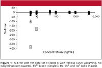
Figure 1

The ΣRE data of Table II summarize the data of Figures 1 and 2. For set 1, the ΣRE drops from no weighting (12.23) to 1/x^0.5 weighting (3.39), then it levels off for additional weighting (not shown larger than 1/x³ ). These results also suggest that 1/x² is the simplest model that adequately describes the curve.

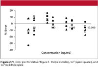
Figure 2

The data of Table II can be used to compare the impact of curve weighting on data sets 1–3 (note that the values of ΣRE are useful for comparisons only within a given data set, not between data sets). In each case, the calibration curve benefits from weighting. For set 2, it appears that 1/x^0.5 should be adequate, whereas 1/x would be appropriate for set 3. Little improvement is obtained with additional weighting for either of these data sets. It is a general observation that bioanalytical LC methods benefit from weighting up to 1/x² . The benefit is further illustrated in the lower section of Table II that compares the LLOQ (±20% limits, with outlier tests to allow discarding one point from the curve) for data sets 1–3 with no weighting and 1/x² weighting. In each case, curve weighting allows a lower value for the LLOQ than when no weighting is used, thus extending the useful range of the method.

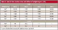
Table II: Sum of the relative error and effect of weighting on LLOQ

Finally, let's examine data set 4. This was used as an example of when to force the calibration curve through zero (x = 0, y = 0) in the first installment of this series (1). There we saw that if the curve was forced through zero, the %-error for the lowest concentration was 45% as opposed to 20% with a nonzero y-intercept. A few readers e-mailed me to ask why I didn't use curve weighting for the treatment of the data. This is a good question, because, as the data of Table II show, curve weighting reduces the ΣRE significantly. The overall result is that with 1/x² weighting, the 20% error observed with no weighting drops to ≤3% throughout the curve. This makes me recall a quote from my favorite statistics book (7, p. 107): "The comments made in the previous section on conventional or unweighted regression calculations indicate that weighted regression calculations should perhaps be adopted far more frequently than is in fact the case."

Summary

We have seen this month that the use of curve weighting can be an effective way to improve the performance of LC method calibration curves. This is summarized nicely in the first sentence of (5): "When the assumption of homoscedasticity [equal standard deviations throughout the curve] is not met for analytical data, a simple and effective way to counteract the greater influence of the greater concentrations on the fitted regression line is to use weighted least squares linear regression." So, although the technique might take a little more work during the calibration process, the payoff usually is worthwhile.

If you would like to read more about curve weighting, reference 5 is an excellent source; an earlier "LC Troubleshooting" column (8) also discussed this topic. Statistics books targeted at the analytical audience, such as reference 7, also contain details about curve weighting, as well as the other topics covered in this series of articles on calibration curves.

John W. Dolan "LC Troubleshooting" Editor John W. Dolan is Vice-President of LC Resources, Walnut Creek, California; and a member of LCGC's editorial advisory board. Direct correspondence about this column to "LC Troubleshooting," LCGC, Woodbridge Corporate Plaza, 485 Route 1 South, Building F, First Floor, Iselin, NJ 08830, e-mail John.Dolan@LCResources.com.

For an ongoing discussion of LC trouble-shooting with John Dolan and other chromatographers, visit the Chromatography Forum discussion group at http://www.chromforum.org.

References

(1) J.W. Dolan, LCGC 27(3), 224–230 (2009).

(2) J.W. Dolan, LCGC 27(4), 306–312 (2009).

(3) J.W. Dolan, LCGC 27(5), 392–400 (2009).

(4) J.W. Dolan, LCGC 27(6), 472–479 (2009).

(5) A.M. Almeida, M.M. Castel-Branco, and A.C. Falcão, J. Chromatogr., B 774, 215–222 (2002).

(6) "Guidance for Industry: Bioanalytical Method Validation," http://www.fda/gov/cder/guidance/index.htm (May 2001).

(7) J.C. Miller and M.N. Miller, Statistics for Analytical Chemistry (John Wiley & Sons, Hoboken, New Jersey, 1984), pp. 102-112.

(8) M.M. Kiser and J.W. Dolan, LCGC 22(1), 112–117.