Looking for New Selectivity in Reversed-Phase Liquid Chromatography? A View of the Selectivity Landscape Over the Past Two Years

The offerings of commercially available columns for reversed-phase liquid chromatography (LC) continue to expand. Are these columns similar or different compared to what is already available?

One of the most common questions practitioners of reversed-phase liquid chromatography (LC) ask is “Which column should I use?” There are over 1000 reversed-phase columns that are commercially available today, and at first glance the prospect of choosing just one, or a few, can be daunting. As I frequently tell my students, the good news is that we have a lot of good columns to choose from, but the bad news is that we have to choose, because it is impractical to evaluate all of them, or even a large subset, for a particular application. A running joke in the community is that the best column for an application is the one that’s already in the laboratory drawer. In other words, column choice is strongly influenced by the experience of the practitioner, and prior good or bad experiences with particular columns. We all have our favourites, and tend to stick with them. A related question is “Does the latest and greatest column from manufacturer ABC really represent a ‘new’ selectivity?” It is difficult to provide a completely satisfying general answer to this question. However, we can leverage existing data to give us some perspective on new phases as they are introduced to the marketplace and we consider adding them to the collections in our laboratory drawers. In this month’s instalment of “LC Troubleshooting”, I provide a perspective on the characteristics of the columns introduced to the commercial market over the last 24 months, using the hydrophobic subtraction (HS) model of reversed‑phase selectivity.

Essential Elements of the Hydrophobic Subtraction Model (HSM) of Reversed-Phase Selectivity

The largest single collection of publicly available data that allows comparison of commercially available columns has been assembled over the past 15 years using the HS model of reversed-phase selectivity. The theoretical foundation of this model, and examples of its application for choosing columns of similar or different selectivities, have been described in detail elsewhere (1,2). Readers interested in learning more about the model itself are encouraged to consult these resources.

The central idea of the HS model is that most of the selectivity of a reversed-phase column, defined here as the ratio of the retention factor for compound X (k_X) to the retention factor of ethylbenzene (k_EB), can be accounted for by the sum of five contributions that are related to different aspects of physicochemical interactions between solutes and the stationary phase. This relationship is shown in equation 1, where the parameters H, S*, A, B, and C account for properties of the stationary phase related to the hydrophobicity of the phase (H), interactions that are size dependent (S*), hydrogen bond donating (A) and accepting (B) properties of the phase, and the ability of the phase to participate in electrostatic interactions with analytes (C). The parameters η, σ, β, α, and κ account for analyte properties that correspond to the column properties. For example, η accounts for the hydrophobicity of the analyte, κ is a measure of the charge of the analyte in solution, and so on.

The column parameters for any reversed-phase column can be determined by experiment using a mobile phase containing acetonitrile and phosphate buffer (see reference 1 for details). The current characterization protocol involves measuring retention factors for 16 probe solutes and regressing those values against the known solute parameters for the 16 probes. Since the beginning of this work in the early 2000s, over 700 commercially available columns have been characterized in this way, and for the last five years the characterization work has been done in my laboratory. These data are accessible through two free, public websites (3,4).

With the column parameters in hand, we can then think about how similar or different any particular pair of columns is. For this purpose, Snyder and Dolan and coworkers have advocated for the use of a “similarity factor”, FS, which is a weighted distance between two columns in five-dimensional selectivity space. The relationship between FS and the column parameters is shown in equation 2:

where X_H, X_S*, etc. are the weighting coefficients with values of 12.5, 100, 30, 143, and 83, suggested by Snyder and coworkers (1). When FS is calculated this way, columns for which FS < 3 are considered “equivalent”, meaning that they are effectively interchangeable, and will produce very similar chromatograms for most applications. Several users have told me that for many applications even FS < 10 is sufficient to obtain very similar separations. Of course, this must be verified experimentally for any particular application, but it is at least a good guideline. Columns for which FS > 100 are considered very different, and looking for such columns may be useful when intentionally assembling a set of columns with very different selectivities. Interpretation of FS values between 3 and 100 depends on the properties of solutes in a particular mixture of interest, and the degree of change in selectivity that is tolerable when trying to identify columns with similar selectivity (or “equivalent” columns) (2).

New Entries in the HSM Database in the Last 24 Months

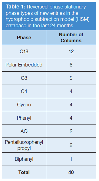
Over the last 24 months, we have made 40 new entries for reversed‑phase columns in the publicly available hydrophobic subtraction model (HSM) database. A summary of the numbers of columns in different phase categories is shown in Table 1. Some of these columns are truly new, both to the database and to the commercial market. Others have been on the market for some time, but have only been characterized by the HSM recently.

What’s New, and What’s Not?

Using the similarity factor (F_S) as a measure of similarity of the new entries to columns already in the database, we can explore a variety of interesting questions.

Question #1: How many of the new entries constitute an addition of a “new” selectivity to the database?

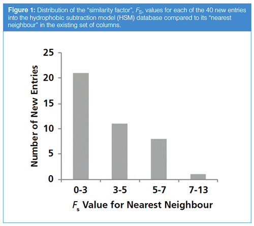
In thinking about this question, I am defining a “new” selectivity as one for which there is currently no equivalent in the database. We can answer this question by taking each new entry, one at a time, and calculating F_S for the comparison of the new entry to all previous entries in the database. If the smallest F_S for all of these comparisons is greater than 3, then the new entry constitutes a “new” selectivity. Figure 1 shows the distribution of the minimum F_S values for each new entry that result from these calculations. We see that, for roughly half of the new entries (21 out of 40), the new entry is “equivalent” to a column that was already in the database (that is, 0 < F_S < 3). This may happen as manufacturers aim to add a column to their portfolio with a selectivity that is similar to a phase that has been quite popular historically. What is perhaps most interesting about this result is that this set of 40 new entries does not contain any selectivities that are radically different relative to what was already in the database. Of the 19 “new” selectivities, the largest minimum F_S value (that is, the F_S value for the new column and it’s “nearest neighbour”) is just 13 out of all the new entries (this particular column is a wide-pore C4 column, if you’re curious). We see that the minimum F_S values for all of the other new entries lie in the range of 3 to 7, which for most applications will be only slightly different relative to other selectivities in the database (2).

Now, I think one could reasonably argue that these results are surprising, but in different directions. On the one hand, we could say that it is surprising that all of the new entries are so similar to existing selectivities. On the other hand, one could say that it is surprising that nearly half of the new entries are unique, because there are only nine phase groups represented in Table 1. In other words, shouldn’t a new pentafluorophenyl (PFP) phase be very similar to an existing PFP phase? Using F_S as a measure of similarity, both of the PFP phases in the group of 40 new entries turn out to be “new” selectivities. How can this be? I actually think that we can explain both apparent surprises by recognizing that the selectivities that populate each phase group are really quite diverse. In other words, one C18 is not necessarily equivalent to the next C18, and one PFP is not necessarily equivalent to the next PFP, even though we talk about them as being the “same” chemistry. This point about the diversity of selectivities within a phase group has been discussed for quite a long time, but I don’t think the extent of the diversity is widely appreciated. Readers interested in the history of this issue, some of the origins of the selectivity diversity, and the consequences for method development are referred to John Dolan’s article on the topic in this column several years ago (5).

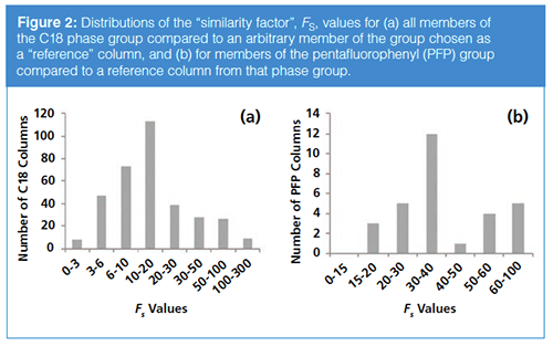
One way to examine this is to look at the distribution of F_S values for all columns within a particular phase group compared to some arbitrary “reference” column within that group. Currently, there are 344 columns in the HSM database that are identified as “C18”, and 31 that are identified as “PFP”. Figure 2 shows the distributions of F_S values for the members of each group relative to a randomly selected member of the same group (that is, the “reference column”). We see that in each case very few columns within a group are similar enough to be “equivalent” to the reference column. In the case of the C18s, just five columns meet that criterion, and in the case of the PFPs the reference column itself is unique! In other words, it is far more likely that any C18 chosen from the group will be different from another member of the group than it is that the two will be equivalent.

Question #2: How many columns that previously had no equivalent in the database now have at least one equivalent due to the addition of the new entries?

The previous question was focused on the extent to which new entries to the database reflect the addition of “new” selectivities. But, this is not the only way to add value to the complement of commercially available phases. New entries that are “equivalent” to columns that previously had no equivalent in the database are also important, because they provide users with alternate columns in case a problem develops with the column originally used to develop a method (for example, if the manufacturer goes out of business, or discontinues the product). Of the 689 columns in the database prior to the addition of the 40 most recent entries, 329 of those were “unique” in the sense that there was no other column in the database with F_S < 3. Of those 329, 322 still have no equivalent column, even after the addition of the 40 new entries. In other words, seven of the 40 new entries fill a role as an “equivalent” for a column that previously did not have one.

Summary

The continuously changing offerings of reversed-phase columns present both opportunities and challenges to practitioners looking to choose a column. On one hand, it is great to be able to choose from over 1000 different commercially available options. On the other hand, it can be difficult to tell whether or not new offerings add truly unique selectivity that we have not seen before. The hydrophobic subtraction model of reversed-phase selectivity is a tool, supported by a freely available database of more than 700 columns, that can be used to answer a variety of questions along these lines. Continued research on this and related models will be important to the community as we look to efficiently develop effective LC methods, even as the number of commercially available columns continues to increase.

References

1. L.R. Snyder, J.W. Dolan, D.H. Marchand, and P.W. Carr, in Advances in Chromatography (CRC Press, Boca Raton, USA, 2012), pp. 297–376.
2. J.W. Dolan and L.R. Snyder, LCGC North Am.34(9), 730–741 (2016).
3. hplccolumns.org, (n.d.). http://hplccolumns.org/index.php.
4. http://www.usp.org/usp-nf/compendial-tools/pqri-approach-column-equiv-tool, (n.d.).
5. J.W. Dolan, LCGC Europe24(3), 142–148 (2011).

Dwight R. Stoll is the editor of “LC Troubleshooting”. Stoll is a professor and co-chair of chemistry at Gustavus Adolphus College in St. Peter, Minnesota, USA. His primary research focus is on the development of 2D-LC for both targeted and untargeted analyses. He has authored or coauthored more than 50 peer‑reviewed publications and three book chapters in separation science and more than 100 conference presentations. He is also a member of LCGC’s editorial advisory board. Direct correspondence to: LCGCedit@ubm.com