How Close is Close Enough? Accuracy and Precision

Modern gas chromatographs are expected to deliver the highest performance levels, but actual performance can suffer because of a number of causes that include poor sample preparation, poor injection technique, incorrect flows or temperatures or inappropriate data handling. Measured performance levels can also vary for samples at different concentrations or containing different chemical substances.

It is always important to keep accurate and complete records of periodic test mixture analyses, any changes to instrument configuration, the methods used and samples run to help diagnose problems when they occur. Sometimes a problem is obvious; often, however, something seems to be going wrong but there is no catastrophic failure. Retention times begin to drift, area counts start to decrease or repeat results seem more scattered than before. Deciding if the changes are significant is a nontrivial task. If there is a significant problem, then further steps can be taken to diagnose and resolve it. If the problem is insignificant, then considerable time might be saved.

Monday Morning Syndrome

Most chromatographers have encountered "Monday morning syndrome" — results obtained at the end of the previous week do not seem to match those acquired on Monday morning. For example, consider the first two columns of Table 1, which give retention time data for one peak in a mixture across 11 consecutive runs. The first ten runs represent data taken on a Friday at 45 min intervals, while the eleventh was the first run on Monday, after a full weekend of instrument idle time. The 14.41 min time obtained on Monday morning is clearly different from the 14.38 min average of the 10 Friday runs. But how significant is this difference? The Monday time lies outside the range of the Friday data, but only by 0.01 min from the longest Friday retention time. Is there a difference, or can this result be expected as part of normal operation? A statistical approach can help answer this question but, as we will see, additional data are required to arrive at a truly meaningful answer.

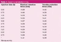
Table 1: Experimental retention times.

A random distribution of data about an average value can be anticipated if the fluctuations in the data are caused by random inlet pressure changes, oven temperature drift, noise-induced data-handling variations, or other system variability. Sometimes the observed fluctuations might exhibit apparent trends, as seems to be the situation in Figure 1, where a sinusoidal trend is evident in the retention data. Is this a real trend or is it just the human eye picking out a pattern where none exists? Even if there is a dependency upon external conditions, the observed retention times in this instance can be considered to be random in the sense that they will tend to group around a central average value, as long as the external causal variables fluctuate around an average value as well.

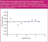
Figure 1

If a large number of random retention times were to be measured, the frequencies with which each retention time occurs could be expected to be grouped around the average value in a more-or-less bell-shaped, or Gaussian, normal distribution curve. The set of 10 Friday measurements represents a small sampling from this hypothetical population of many values, but this is all the data that we have. Using statistical analysis, we can infer the properties of the large hypothetical population of retention time measurements from our sample data set. Then, we should be in a position to compare the anticipated behaviour with other experimental data.

The degree of scattering of random data can be expressed in terms of its standard deviation, and the location of the data can be expressed by its average. In a normal distribution, approximately two-thirds of the data points will lie within one standard deviation (s) to either side of the average (y bar), and about 95% of the points will lie within two standard deviations. The experimental average and standard deviation can be calculated from the data according to the following equations:

where y_i represents the ith experimental value and n is the number of samples. For the set of Friday data in the second column of Table 1, the average, y bar, equals 14.38 min and the standard deviation, s, equals 0.011. The frequency of each retention time in the first column of Table 1 is plotted in Figure 2, along with an ideal normal distribution function that has the same average and standard deviation as the observed data set.

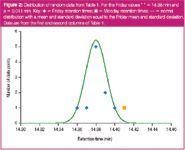
Figure 2

Visual evaluation of Figure 2 shows that the Monday retention time does not seem to fit in with the collection of Friday data; the Monday point lies slightly outside of the normal distribution curve for the Friday data. We can quantify this assessment by calculating the difference between the Monday morning retention time and the Friday average, in terms of the standard deviation. According to Equation 3, this value equals (14.41 – 14.38)/0.011 = 2.73 standard deviations away from the average value. More than 99% of the points in a normal distribution lie within 2.7 standard deviations of the average, so on this basis, there is less than a 1% chance that the Monday morning point fits into the set of Friday data.

To make the foregoing conclusion, we have relied upon several important assumptions. First, when constructing the normalized distribution curve in Figure 2, we assumed the (hypothetical) population standard deviation, σ, that would be obtained from a large number of retention-time measurements was equal to the experimental standard deviation, s, of the measured retention time data. We also assumed that the mean value of the population of all retention time measurements, η, is equal to the average of our limited set of 10 measurements, y bar. In reality, however, the experimental average and standard deviations are merely estimates of the hypothetical population's characteristics. The more samples we acquire, the better the estimates become. But with only a small number of available measurements, we are at risk of making the wrong conclusion based upon a normal distribution curve because of this imprecision.

A related family of distribution curves, called Student's t-distribution after the author's pseudonym used in its first published description in 1908, extends the expected probabilities of obtaining a particular result to accommodate small sets of characterizing measurements, typically 5–25 samples, and the concomitant uncertainty of the standard deviations they represent. As the number of samples increases, the t-distribution's shape in its leading and trailing tail areas approaches the normal distribution. Families of t-distribution curves are given in tables in statistical books as well as in spreadsheet programs.

To apply the t-distribution to the evaluation of a specific observed value y_obs, we can substitute the known standard deviation — as calculated from the experimental data — for the estimated population standard deviation in Equation 3 to give Equation 4:

and then compare tobs with the t-distribution curve that corresponds to a sample size of 10.

Statisticians speak of the number of degrees of freedom in a data set, which is equal to n – 1 in situations such as this retention time data. A degree of freedom implies that the data are free to change as they are collected. There are only nine degrees of freedom in ten samples because, in truly random data, the differences between each sample value and the population average value must add up to zero. If the population average value is known, then one of the ten sample values is predetermined by the other nine. Tables of the t-distribution usually list probability values in terms of the number of degrees of freedom in a data set.

The Monday result lies 2.73 standard deviations away from the average, and with nine degrees of freedom in the base data, the t-distribution gives a greater than 98% probability that the Monday time does not belong in the set of Friday times. This is somewhat less than the 99+% probability deduced from the normal distribution curve, and it reflects the fact that the standard deviation of the Friday retention data is really only an estimate of the standard deviation that would characterize a much larger set of retention data — such estimates from small data sets usually overestimate the population standard deviation. If we had obtained a larger number of retention time observations in the Friday data, then the error in the corresponding estimate of the population standard deviation would decrease, and the probability given by the t-distribution evaluation of the Monday result would approach the value predicted by using the normal distribution code.

Note the assumption that η = y bar; the data that are used to calculate s are assumed to be normally distributed around the average value. The assumption of randomness is very important when assessing data in this manner; it implies that each successive measurement does not depend at all upon the previous measurements; that all the values are, in essence, random draws out of a "hat" that contains all possible retention times for that peak under those conditions. If instead the retention times steadily increase or decrease from run to run, then calculations based upon simple statistics of this type are not very meaningful.

The conclusion that there is a 98% probability that the Monday retention time does not belong with the group of Friday measurements is a relatively weak one. A single measurement of this type, especially coming after an extended idle period on a gas chromatography (GC) instrument, might be anticipated to lie outside of the distribution of data from a previous day. Certainly most experienced chromatographers would not consider this situation unusual. A better approach to this question is to continue running the instrument on Monday and collect a new series of measurements for comparison to the Friday data set.

Trends in the Data

The influence of laboratory temperature, for example, on retentions measured over one or more days can be essentially random — assuming that the air conditioning functions normally — but often this is not the situation with other types of external influences. A steadily increasing septum leak, for example, can cause peaks' retention times as well as areas to drift in a defined direction as the leak worsens from one injection to the next. The third column in Table 1 shows some retention data with a discernible trend towards increasing retention times as the total number of runs increases; these trending data are plotted in Figure 3, where it seems fairly obvious that retention times are increasing. Because of this, we can no longer use the previous statistical approach to characterize the data. The data are no longer entirely random: each subsequent run has, on average, a slightly longer retention time, and so the data violates the previous assumption that they are distributed randomly around an average value. Instead, retention times from the beginning of the experimental measurements are generally shorter than those obtained towards the end. The average value of any sequential subgroup of this data will depend upon the time interval over which the subgroup was collected.

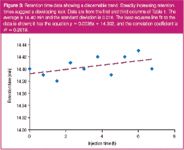
Figure 3

The influence of apparent trends like this can be evaluated by performing a linear least-squares procedure to fit a line to the data. The slope of the estimated line and a measurement of the randomness of the data in relation to the line can help decide if a meaningful trend is present in the data. Equations for such calculations take many different forms; Equations 5–7 show some examples. Fortunately, such calculations are available in spreadsheet programs as well as in a number of web-page applications. The equations attempt to find the line that has the least error when compared to the data set. The slope of the fitted line, m, is a function of the differences between the data values and their averages; the y-intercept, b, can be calculated from the averages of the data; and the regression coefficient, r², is a more complex function of various sums and differences in the data that characterizes the goodness of fit of the data to the line.

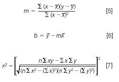
Both Figure 1 and Figure 3 include least-squares lines that have been fitted to their respective data and the coefficients from Equations 5–7 are given in the figure captions. For the random data in Figure 1, the slope of the fitted line is nearly zero, which indicates that there is little dependency between the time of the GC run and the measured retention time of the peak. The regression coefficient is very small as well, which supports the hypothesis that this data set is truly random. The data in Figure 3, however, has a finite slope of 0.0036 min/h, and the regression coefficient is much larger at 0.26. Taken together, these statistics imply that there is a correlation between measured retention times and the time of injection, but also that the data are significantly scattered around the trend line. If the data were to lie in a perfectly straight line, the regression coefficient would be equal to 1.0.

Conclusion

In terms of the Monday morning question that we started with, in the instance of the second, trended set of data, the Monday retention time of 14.38 is neither consistent nor inconsistent with the septum-leak hypothesis. Again, it seems prudent to acquire additional data during the day on Monday and then compare that data to Friday's. From a practical point of view, of course, testing the septum leak idea by using a helium leak detector at the injector nut or, even better, replacing the septum on Mondays or more frequently are very viable alternatives to a laborious study of retention time behaviour. In other instances, such as trying to understand variability in analytical concentrations across a series of runs, from one instrument to another, or from one laboratory to another, the basic statistical analyses present in this article are a good starting point.

"GC Connections" editor John V. Hinshaw is senior staff engineer at Serveron Corp., Hillsboro, Oregon, USA and a member of the Editorial Advisory Board of LCGC Asia Pacific.

Direct correspondence about this column to "GC Connections", LCGC Asia Pacific, Advanstar House, Park West, Sealand Road, Chester CH1 4RN, UK, e-mail: dhills@advanstar.com

For an ongoing discussion of GC issues with John Hinshaw and other chromatographers, visit the Chromatography Forum discussion group at http://www.chromforum.com