Screening Designs (Part 1) — Types and Properties

Screening designs are used to screen for important factors during method optimization or in robustness testing. Usually, two-level screening designs, such as fractional factorial and Plackett–Burman designs, are applied. This column discusses the properties of these designs.

The use of screening designs in method optimization and robustness testing has been mentioned in previous columns.^1,2 They are applied to screen for important factors (i.e., factors with a large influence on the response(s) of the considered method).

Two-level screening designs, such as fractional factorial and Plackett–Burman designs, are usually applied for these purposes.^3,4 These designs allow the effects of a relatively high number of factors, in a relatively small and feasible number of experiments, to be evaluated. This column investigates the properties of these designs and other related concepts, such as interaction effects, contrast coefficients, confounding of effects, generators, aliases, defining relations and design resolution. The analysis of the results of those screening designs will be discussed in more detail in Part II.

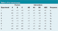
Table 1: 23 full factorial design.

Two-Level Screening Designs

Full factorial designs: To be able to explain the properties of fractional factorial designs, the full factorial designs need to be considered first. A full factorial design contains all possible combinations (L^f ) between the different factors f and their levels L, with L = 2 for two-level designs.³ For example, in Table 1, a 2³ full factorial design for three factors (A,B,C) at two levels (–1 and +1) is shown. The influence of a factor X on the response y is estimated by its effect, E_x, which is equal to the difference between the mean responses with X at (+1) level, ΣY mean (+1), and at (–1) level, ΣY mean (–1). For example, the effect of factor A from Table 1 is given by

A full factorial design also allows the interaction effects between the factors to be estimated. For example, from the design in Table 1, three two-factor interactions (AB, AC, BC) and one three-factor interaction (ABC) effect can be estimated.

In general, a p-factor interaction effect occurs when the effect of a given factor (p = 2) or of a (p–1) factor interaction effect (p > 2) depends on the level of another factor. For a two-factor interaction AB, it means that the effect of A depends on the level of B and vice versa.

Suppose, for example, that A and B are pH and % of modifier in the mobile phase, respectively. An interaction effect occurs when the effect of the pH on the response depends on the fraction of the modifier. As another example, suppose factor B is the HPLC column [with columns C₁ and C₂ as (+1) and (–1) levels, respectively] and factor A is the pH of the mobile phase [with 3 and 9 as (+1) and (–1) levels, respectively]. A two-factor interaction between the column and the pH of the mobile phase occurs when the effect of the pH on the response (e.g., resolution) is different on both columns. The interaction in the latter example is called the pH by column interaction and is symbolized by pH × column, A× B, AB or BA.

From a 2^f full factorial design, the number of different p-factor interactions is equal to

For example, from a 2⁷ full factorial design requiring 128 experiments: 7 main effects, 21 two-factor, 35 three-factor, 35 four-factor, 21 five-factor, 7 six-factor and 1 seven-factor interaction(s) can be estimated.

The interaction effects are calculated by applying the so-called columns of contrast coefficients. They are also shown in Table 1 for the 2³ full factorial design. The contrast coefficients for the interactions in full and fractional factorial designs are obtained by multiplying the levels of the corresponding factors, according to the regular algebraic rules [Table 2(a)].

Table 2: Algebraic rules applied for the columns of contrast coefficients in (a) full and fractional factorial and (b) Plackett–Burman designs.

For example, the levels for AB are obtained by multiplying those of columns A and B for each experiment. Then, the interaction effects are calculated analogously to the main effects. Thus, the interaction effect AB from Table 1 is estimated by

Fractional factorial designs: The main drawback of full factorial designs is that the number of experiments increases exponentially with the number of factors. For example, for 6 factors 64 experiments are required and for 7 factors as much as 128. In practice, performing that many experiments is not feasible. Therefore, often only a fraction of the full factorial design is performed, which is called a fractional (or partial) factorial (FF) design.

Let us first consider a half-fraction factorial design, where only half of the full factorial experiments are performed. For example, for four factors,

experiments are required.

A 2⁴ full factorial design is shown in Table 3. Selecting eight appropriate experiments results in a half-fraction factorial design, symbolized as 2^4–1 . The experiments 1, 4, 6, 7, 10, 11, 13 and 16 (between brackets) constitute a first half-fraction, while the remaining experiments (2, 3, 5, 8, 9, 12, 14 and 15) represent a second half-fraction.

Table 3: 24 full factorial design, with indication of two half-fraction designs.

Obviously, reducing the number of experiments leads to a loss of information that can be gained from the design. Contrary to a full factorial from an FF design, not all main and interaction effects can be estimated individually anymore. For example, consider the first half-fraction design from Table 3 (experiments in brackets). The columns of contrast coefficients for the three-factor interactions [Table 4(a)] show that column ABC is equal to D, ABD to C, ACD to B and BCD to A. In fact, from this design, when estimating the effect of factor D, the summed effects of D and ABC are obtained. In other words, D and ABC are confounded (i.e., they cannot be estimated separately anymore).

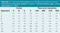
Table 4(a): 24–1 half-fraction factorial design (from Table 3) and the columns of contrast coefficients for the three-factor interactions. and (b) 24–1 half-fraction factorial design, created using generator D = ABC.

Analogously, all other factors are also confounded with a three-factor interaction (A with BCD, B with ACD and C with ABD). Similarly, from the contrast coefficients for the two-factor interactions (not shown), it would be observed that they are confounded among each other in this design, (e.g., AB with CD). In summary, an estimated effect is always the sum of two effects in a half-fraction design.

The magnitude of main effects tends to be larger than two-factor interactions, which in turn tend to be larger than three-factor interactions, and so on. Thus, in the half-fractional factorial design of Table 4, the main effects are expected to be considerably larger than the three-factor interactions with which they are confounded, or, in other words, the three-factor interactions are considered negligible to estimate the main effects. Consequently, the estimate for the main effect in such a design is still supposed to be a proper one.

In practice, a half-fraction design is not selected from a full factorial, as described above, but constructed independently. To construct a 2^4–1 FF design, first a full factorial design for 4 – 1 = 3 factors is built [see Tables 1 and 4(b)]. Then, the fourth factor D is awarded to one of the interaction columns [e.g., to ABC, see Table 4(b)]. Thus, factor D will be confounded with the interaction ABC and a design equivalent to the one in Table 4(a) is obtained.

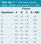
Table 4(b): 24–1 half-fraction factorial design, created using generator D = ABC.

The relationship D = ABC is called the generator of the design. The factor D and the three-factor interaction ABC are called aliases of one another, because they are confounded. All aliases in an FF design can be derived from its so-called defining relations or defining contrasts (I). In a half-fraction design, only one defining relation exists, which is obtained by multiplying or combining both terms of the generator (Equation 3).

The aliases of each factor or interaction can be derived by combining it with the defining relation, with the additional rule that any term appearing an even number of times disappears from the result. For example, the aliases of A (i.e., BCD) and of AB (i.e., CD) are determined as in Equations 4–5.

The design resolution is determined by the (smallest) number of terms in the defining relation(s). The higher the design resolution, the higher the order of the interaction effect(s) that is/are confounded with a main effect. Generally, with a design resolution equal to R, a factor is confounded with interactions containing at least R–1 terms, or no p-factor (interaction) effect is confounded with any effect containing less than R–p factors. The design of Table 4 is, therefore, called a design of resolution IV, and is symbolized as a 2^4–1 (IV) design. No main effect (p = 1) is confounded with an interaction of less than three factors (R–p = 3) and no two-factor interaction (p = 2) is confounded with an interaction of less than two factors (R–p = 2).

Often a half-fraction factorial design still requires too many experiments and then smaller fractions of the full factorial are executed. Such fractions result in, for instance, quarter-fraction, eighth-fraction or sixteenth-fraction factorial designs.

Let us, for example, construct a quarter-fraction factorial design for six factors, symbolized by 2^6–2 , applying the above approach. Only one fourth of the experiments from the full factorial design (i.e.,

experiments) are required. The first four columns (A, B, C, D) are constructed as the full factorial design for four (i.e., 6 – 2) factors (Table 5). For the last two columns (E,F), generators must be defined. The choice is free and up to the analyst, for example E = ABCD and F = ABC is a possibility. The generators lead to two defining relations, I = ABCDE and I = ABCF. In fact, in a quarter-fraction factorial design, each effect is confounded with three others. Determining the confounding pattern thus requires three defining relations. The third (Equation 6) is derived from multiplying the two relations obtained from the generators, using the rules applied in Equations 4–5.

The resolution of the design with the above generators is III, since the smallest defining relation contains three terms. Consequently, certain main effects are confounded with two-factor interactions (e.g., D = EF = ABCE =ABCDF).

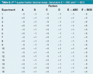
Table 5: 26–2 quarter-fraction factorial design. Generators E = ABC and F = BCD.

Because two-factor interactions tend to be larger than three-factor interactions, it is preferred to construct a design with resolution IV (or even higher), when this is possible for a given number of experiments. With resolution IV, the main effect is confounded only with three-factor and higher-order interactions. Such a design is expected to result in better estimates for the main effects, than the above design with resolution III. For example, selecting the generators E = ABC and F = BCD for the 2^6–2 design leads to resolution IV. The defining relations then are I = ABCE, I = BCDF and I = ADEF. The thus constructed design is shown in Table 5.

Analogously to the above procedure, smaller fractions of a full factorial design can be constructed. The defining relations are obtained by making all possible multiplications between the defining relations derived from the generators. Suppose an eight-factor sixteenth-fraction factorial design is created. To construct such a 2^8–4 design, four generators need to be defined, resulting in four defining relations. The number of confounded effects is sixteen and the number of defining relations fifteen. The eleven missing relations are obtained as follows. Multiplying the four original two by two leads to six new relations, and three by three produces four new relations, while multiplying them four by four results in the final relation.

Generally, a two-level fractional factorial design 2^f–ν examines f factors, each at two levels, in 2^f–ν experiments, with ½^v the fraction of the full factorial (ν = 1, 2, 3,...). A fractional factorial design always requires a number of experiments that is a power of two. Those with eight or sixteen experiments are executed most frequently. To construct such designs, ν generators need to be defined. In a 2^f–ν FF design, each effect is confounded with 2^ν–1 other effects. The design is characterized by a total of 2^ν–1 defining relations.

The smallest fraction from which the main effects can still be estimated unconfounded from each other is called a saturated fractional factorial design. For example, the 2^7–4 design allows estimating seven factor effects from eight experiments. In these designs, the resolution is III (i.e., the main effects are confounded with two-factor interactions).

Plackett–Burman Designs

Plackett–Burman (PB) designs are considered the main alternative for saturated fractional factorial designs. PB designs are saturated factorial designs of resolution III that examine N–1 factors in N (a multiple of four) experiments.⁵ They only allow the main effects to be estimated. Designs for N up till 100 are described, although those with more than 24 experiments are usually practically not feasible. Most commonly applied are those with 8, 12 or 16 experiments. For example, in Table 6, a PB design that allows 11 factors to be examined in 12 experiments is shown.

To construct Plackett–Burman designs, the first line, given by Plackett and Burman,⁵ is used for the factor levels of the first experiment. Below, the first lines are given for PB designs with N = 8, 12, 16, 20 and 24 experiments.

The signs + and – represent the (+1) and (–1) levels, respectively (see Table 6). Then, the following N–2 rows are obtained by a cyclic permutation with one place compared to the previous row. The sign of the first factor (A) in the second row becomes equal to that of the last factor (K) in the first row. The signs of the following N–2 factors in the second row are equal to those of the first N–2 factors of the first row (see Table 6). The third row is derived similarly from the second. This procedure is performed N–2 times, and finally, a last N^th row of minus signs is added.

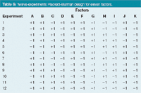
Table 6: Twelve-experiments Plackett–Burman design for eleven factors.

Since PB designs have resolution III, two-factor and higher-order interactions are confounded with the main effects. For example, in the N = 8 PB design, each main effect is confounded with fifteen higher-order effects, among which three two-factor interactions. The PB designs with a number of experiments that is a power of two are equivalent to fractional factorial designs. The confounding of a given interaction with a factor can be derived from the columns of contrast coefficients. However, different algebraic rules are applied for PB designs [see Table 2(b)]. In fact, the rules are opposite to those for the FF designs. In the other PB designs (e.g., N = 12 or 20), the confounding pattern is more complex and can be considered outside the scope of this column.

A PB design can examine N–1 factors in N experiments, which is different from a fractional factorial design. Some of the FF designs also contain N–1 factors (e.g., the 2^7–4 design). However, this is usually not the case (e.g., the 2^5–2 or 2^6–3 designs).

When the number of factors to be examined is lower than N–1, then the remaining columns in a PB design are defined as dummy factors. A dummy factor is an imaginary variable for which a change in its levels does not correspond to any physical or chemical change. A dummy is awarded arbitrarily or randomly to a given design column. Whereas a fractional factorial design is constructed based on the number of factors to be examined and no dummies are entered in those designs. The difference is illustrated by the following example. To examine six factors, for example, PB designs with N = 12 and 5 dummies, or with N = 8 and 1 dummy can be applied. For the same purpose a 2^6–3 FF design could be chosen (generators D = BC, E = AB, and F = AC) with eight experiments, similar to the N = 8 PB design, but containing no dummies.

Three-level screening designs

Occasionally, a screening at three levels (–1, 0, +1) is executed. Only a limited number of three-level screening designs are described, for example, N = 9, f = 4 (Table 7) and N = 27, f = 13.⁶

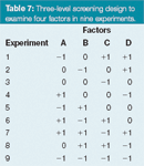
Table 7: Three-level screening design to examine four factors in nine experiments.

Another possibility is provided by the so-called reflected designs. Reflected designs are in fact full factorial, fractional factorial or Plackett–Burman designs that are duplicated [i.e., executed once with the factor levels (–1, 0) and once with (0, +1)]. These designs require 2N–1 experiments to examine f factors, because one experiment in both N-experiments two-level designs is common. For example, to examine seven factors at three levels, fifteen experiments are needed when constructing a reflected design from a N = 8 PB or a 2^6–3 FF design.

Bieke Dejaegher is a postdoctoral researcher at the same department as Yvan Vander Heyden, working on experimental designs and their applications in method development and validation.

Yvan Vander Heyden is a professor at the Vrije Universiteit Brussel, Belgium, department of Analytical Chemistry and Pharmaceutical Technology, and heads a research group on chemometrics and separation science.

References

1. Y. Vander Heyden, LCGC Eur., 19(9), 469–475 (2006).

2. B. Dejaegher and Y. Vander Heyden, LCGC Eur., 19(7), 418–423 (2006).

3. Y. Vander Heyden, C. Perrin and D.L. Massart, Optimization strategies for HPLC and CZE, in K. Valko (Ed.), Handbook of Analytical Separations 1, Separation Methods in Drug Synthesis and Purification, Elsevier, Amsterdam, pp. 163–212 (2000).

4. Y. Vander Heyden et al., Journal of Pharmaceutical and Biomedical Analysis, 24, 723–753 (2001).

5. R.L. Plackett and J.P. Burman, Biometrika, 33, 302–325. (1946)

6. Y. Vander Heyden, M.S. Khots and D.L. Massart, Analytica Chimica Acta, 276, 189–195 (1993).