Sampling: The Ghost in Front of the Laboratory Door

Sampling can be the most demanding part of an analysis. Anybody in charge of sampling needs a good understanding of the composition of the material to be investigated, its heterogeneity (or homogeneity, in simple cases), and the chemical properties of the analytes. Sampling procedures must be described in detail. Detecting the bias of a sampling procedure can be difficult; this fact is trivial, but it must not be forgotten. In many cases, gaseous and aqueous samples are homogeneous, at least at the local scale, but most solid samples are heterogeneous. A typical example is soil, which presents a twofold demanding problem for the analyst: first, the selection of the sites where the samples are taken, and second, the reduction of a sample (for example, 1 kg) to the analysis size (for example, 10 µL). The greater the heterogeneity of a material, the deeper a knowledge of sampling statistics is needed. In demanding cases, one should not do the work without the advice of a statistician.

Analytical laboratories must follow various guidelines, such as ASTM standards, ISO norms, methods defined in pharmacopeias, good laboratory practices (GLPs), in‑house standard operating procedures (SOPs), and so on. The responsibility of the analyst is often restricted to the professional execution of well-validated analyses, as required by the ordering party. In such cases, one is not bothered with sampling. But even then, it is obvious that all efforts to obtain true and precise analytical results (whereas trueness is more important than precision) are of little relevance if the sampling process was erroneous. The repeatabilities of the injection, of the method, or of the sample preparation have nothing to do with the pitfalls of sampling. For sample preparation in chromatography, see the book by Moldoveanu and David (1).

Sampling can be easy and almost error-free, or it can be difficult and error-prone. Concerning its errors, we can distinguish sampling bias and sampling uncertainty. Sources of bias include, but are not limited to:

• Wrong probing, such as taking samples only from the surface of the test piece, or only from well-accessible places.

• Wrong containers, which contaminate or alter the samples during storage (2) and transport. Acidic solutions could dissolve cations from metallic boxes.

• Containers that are not airtight, which can lead to evaporation of water or compounds with a high vapour pressure.

• Too high a storage temperature, which could induce chemical decomposition of the sample.

• Sources of uncertainty can be, but are not limited to:

• Large but underestimated heterogeneity of the material; as a consequence, too small a number of samples is taken.

• Lack of knowledge of the sample composition. Maybe there are complexing agents that hide a certain amount of cations, or one does not know at all what might be present in the sample. It might be a party drug that is unknown so far; in that case, a quick test will not find it. If a high content of glycerol is not expected in wine, it is very possible that such a fraud will not be detected.

In some cases, it can be very difficult or impossible to detect (or assume) both bias and uncertainty. If a high degree of heterogeneity is presumed, the number of samples to be taken must be high. Usually, the heterogeneity of solid samples is of greater concern than that of gases and liquids.

However, there are also cases with simple and unambiguous sampling. If a doctor or nurse is taking blood from a person, everybody agrees that (a) this (perhaps tiny) sample represents the health state of the day, and (b) the analytical result is accurate, because it is obtained by a validated and well-maintained device for clinical analysis.

In any case, the sampling procedure must be described in detail, including its possible pitfalls. If the material in question is heterogeneous, the uncertainty of sampling may be high, and this fact needs to be mentioned in a clear way.

The “great old man“ of sampling was Pierre Maurice Gy. He wrote numerous books about this topic, and their content is only readable for specialists ([3,4] as examples). Fortunately, there exists an easy-to-understand summary of his work by Patricia L. Smith (5). Her 96-page book presents not only Gy’s error theory, but also simple experiments for its clarification.

IUPAC published a general sampling nomenclature for analytical chemistry in 1990 (6), and a terminology recommendation for soil sampling in 2005 (7).

Example of a Simple Gaseous Matrix: Air Pollution

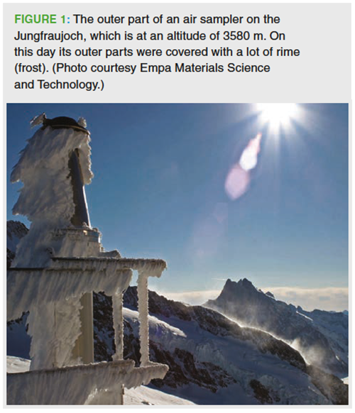
The sampling problem of this example is simple because the sample is homogeneous at the local scale, although it is heterogeneous at the continental scale. Graziosi and associates investigated the carbon tetrachloride emissions in Europe (8), a long-lived greenhouse and ozone‑depleting compound. What was needed were samplers (linked to analyzers such as gas chromatography–mass spectrometry [GC–MS] instruments, located at different places within Europe), meteorological data, and statistical analysis. One of the sampling places was the Jungfraujoch, which is at an altitude of 3580 m in the Swiss Alps (Figure 1). Continuous sampling over years allowed the identification of “emission hot spots“ of CCl₄. They were found in southern France, central England, and the Benelux countries (Belgium, Netherlands, Luxembourg). The good news is that the CCl₄ emissions are decreasing, at least in Europe; the bad news is that they are still too high.

Example of a Simple Liquid Matrix: Water Pollution

This case is similar to the air pollution problem. A continuous high-resolution liquid chromatography–tandem mass spectrometry (LC–MS/MS) survey of Rhine river water at Weil (Germany) showed an unknown large peak in June 2016 (9). Sampling was easy, due to the locally homogenous character of the sample, but revealing the mystery was not. Upstream sampling at different places led to the conclusion that the source was in the region of Säckingen or Stein. A chemical plant was identified as the polluter. A so far unknown by‑product of a synthesis had found its way to the Rhine, amounting to 1.1 tons within one month. The company was cooperative, and modified the process, and was able to eliminate the pollution.

Lakes, however, often need another sampling technique. For the investigation of some environmental problems, samples must be taken at different depths because lakes are stratified (10). At a given depth, a sample is looked at as homogeneous.

A Special Case with Well‑Defined Solid Items: Uniformity of Content

Many drugs are prepared as well‑defined dosage units, namely tablets and capsules, but also powders or solutions that are enclosed in unit-dose containers. Decades ago, the content of the active ingredients was analyzed by taking, for example, 10 tablets, grinding them all together, and determining the mean values. However, as a patient, one wants some guarantee that every single tablet contains the amount(s) claimed on the label, especially if the prescription is one tablet per day. Therefore, the uniformity of content of such drugs needs determination by investigating individual tablets or dosage units. The pharmacopeias require very detailed tests and statistical calculations regarding the uniformity of content, with some minor differences in the procedures as described in the United States (11), European, and Japanese Pharmacopeias. The uniformity of content must be determined for each batch.

Sampling for the uniformity test is simple; however, an interesting detail is noted in the instructions. No fewer than 30 units must be selected, and 10 units of this larger quantity are analyzed individually. Then the acceptance value is calculated with statistical tests explained in an extensive table. If the requirements are not met, the next 20 units are investigated individually, followed by the appropriate statistical test, which is then crucial for acceptance or rejection of the batch.

Less Defined Sampling Units: Sugar Beets

A heap of sugar beets is not a homogeneous material in the strict sense. On the other hand, the heterogeneity is very clear. The heap consists of air, dirt, maybe stones, and beets, but the latter are very similar among each other. The farmer is paid in accordance to the quality of the delivered beets with regard to soiling with dirt, sugar content, α-amino nitrogen, sodium, and potassium.

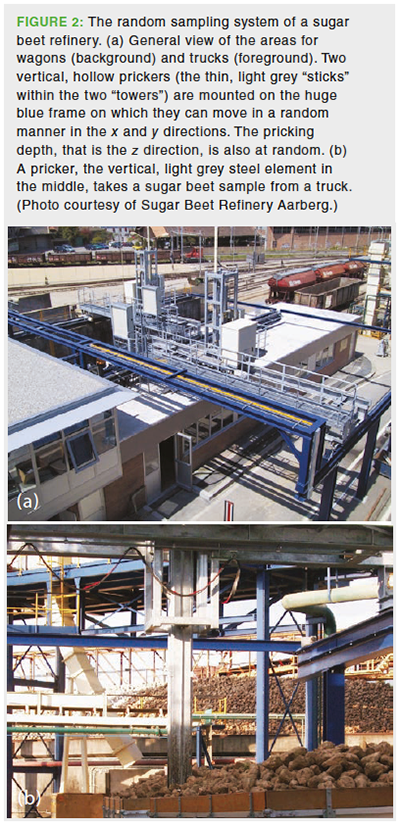
Sugar beets are delivered by trucks or by rail. A typical truck load has a weight of 20 tons, whereas a rail wagon carries about 55 tons (data from the sugar beet refinery Aarberg, Switzerland). From a truck, only one sample of about 30 kg is taken; from a wagon, two samples go to analysis. The samples are taken by a pricker with random steering (see Figure 2 and its legend for construction details as installed at the Aarberg refinery). This approach guarantees that random samples are obtained (see the next section about soil sampling), and that the farmer has no influence on the quality control. There is the risk that a farmer is under- or overpaid because a random sample may not represent the mean quality of his beets. However, most sugar beet farmers have a contract with the refinery over years, and inaccurate payments will equalize over time.

A Difficult Solid Matrix: Soil

Soil is very heterogeneous with regard to the chemical composition of small individual samples, but also with regard to the size of its particles (from dust to large stones). An erroneous soil analysis can lead to wrong and costly decisions: If the concentration of copper, for example, is claimed to be higher than it actually is at a promising site, the investment of a mining company will be in vain. Old advice is still valid:

The intensity with which a soil must be sampled to estimate with given accuracy some characteristic will depend on the magnitude of the variation within the soil population under consideration. The more heterogeneous the population, the more intense must be the sampling rate to attain a given accuracy (12).

In many cases of soil analysis (and of other heterogeneous bulk materials), the uncertainty resulting from sampling will be greater than the uncertainty of the analysis itself.

How does one take representative soil samples if it must be assumed that the distribution of the analytes is not homogeneous over the area in question? The amount of material needed in the laboratory is much smaller than the amount that should be dug in the field. The first step will be to divide the area into (probably rectangular) units of equal size, and to number them consecutively. Afterwards, the units that will be sampled are determined by random numbers (12). It is really important to work with random numbers, and not with some preferences or clever ideas of the analyst. Random numbers can be obtained in a most convenient way from www.random.org (13), which generates true random numbers based on atmospheric noise. Alternatives are the random number function of Excel (less recommended because the results are determined by an algorithm) or a drawing process. An example:

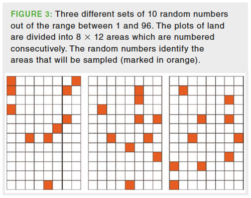
The person in charge decided intuitively to divide the area to be investigated into 96 rectangles. They are numbered consecutively (If the soil is stratified and needs a thorough investigation, the arrangement of numbering must be extended to the third dimension, for example, to volumes instead of areas.) In this example, it was decided to analyze 10 units. At www.random.org, select the free service “numbers,“ and then the random sequence generator (this generator will not present duplicates, as could be the case with the integer generator). The boundaries will be 1 and 96 in this example. Take the first 10 numbers. One may get:

15 92 46 64 69 80 20 9 34 81

Figure 3 shows three different sets of 10 numbers out of 96, as obtained by the random number generator mentioned above. It is obvious that true randomness is much more accidental than our imagination thinks.

From all these sub-fields, a sample, of perhaps 1 kg, is taken. What happens with them in the laboratory? First, the particle size must be reduced by crushing, milling,
or grinding; what should be obtained is a powder of uniform and small particle size (14). Still, and irrespective of the approach (10 samples of 1 kg or a 10-kg mix of all samples), the amount is too large. An old method that can be used is coning‑and‑quartering (15). The material is poured onto a flat surface, then vertically (in the x and y directions) cut into four equal parts, and two opposite parts are processed further, maybe again by quartering. The weak point of this procedure is the fact that pouring will yield a cone with low-density material on the top and heavier particles below; however, not in a regular manner. Therefore, more sophisticated techniques, using specialized machines, are needed for sample reduction.

Despite all these efforts, it is still questionable whether the small amount of the reduced sample that goes to the analysis is representative for the soil to be investigated. The sampling error depends on the number of particles in the sample (15); this fact is the reason why the particle size of the ground material should be as small as possible. The final sample should contain at least 105 particles, but 10⁶ to 10⁷ would be better.

A paper by Walsh and associates discusses the problems associated with the analysis of 2,4-dinitrotoluene in firing point soils and offers interesting reading (16). Sampling of particulate material is the topic of a chapter in a book by Merkus (17).

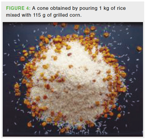
A simple experiment shows that it is difficult or impossible to obtain a representative sample from a heterogeneous mixture of items with different size, such as a material that was not ground to equal particle size. One kg of rice was thoroughly mixed with 115 g of grilled corn in a steel bucket, then poured to a cone, as mentioned above. The result is shown in Figure 4. The larger corn grains are overrepresented at the bottom circumference of the cone (its inner composition is unknown). In addition, their enrichment depends on the direction of pouring. Quartering of the cone of Figure 4 could perhaps be successful, but the result would strongly depend on the orientation of the quartering cross section. The segregation effect that occurs when a mixture with grains of different size (and the density or surface property) is shaken is called the Brazil nut effect (18); large grains accumulate on the top (however, also the contrary can occur which is known as the reverse Brazil nut effect).

Sampling Statistics

A company or laboratory confronted with difficult sampling problems needs deeper knowledge, such as a person who is able to set up sampling plans that follow the rules of state-of-the-art statistics (19).

The two basic rules for correct sampling are as follows (5):

• Every part of the lot has an equal chance of being in the sample. This is why the use of random numbers is important.

• The integrity of the sample is preserved during and after sampling.

It is obvious that even the best sampling plan will yield probabilities, and not certainty. Every analyst, contractor, and customer must live with this fact. Agreement with a limited statistical certainty P, often 95%, is a prerequisite. The number of samples n needed for a confidence interval d and a standard deviation s of the analytical results can be estimated as follows (1):

where t is the variable of Student’s t distribution (20), which can be found in any statistics book. If P = 95.0% and n is high (for example, greater than 20), t rapidly converges towards 2. The problem with equation 1 is the fact that n is unknown, while t depends on n. An iterative process could be needed; however, a good judgement by eye will solve the problem. An example:

The mean m of n = 10 samples is 273 with a standard deviation s = 33 (of a certain analyte such as nitrate or lidocaine, in ppm or another unit). The required statistical certainty P is 95%. t_9,0.95 taken from a Student table is 2.26. The confidence interval d, which represents the tolerable uncertainty in the estimation of m is 15 (a range of m between 258 and 288). Therefore:

Ten samples are not enough for the requirements defined above. If n would be 20, t_19,0.95 is 2.09, and equation 1 gives n = 21. This result means that at least 20 samples should be investigated. Note that even then there is still a 5% risk that the true mean lies beyond the confidence interval of ±15.

The 20 analyses will probably yield another mean and standard deviation than the 10 first ones. Generally, it must not be forgotten that standard deviations from too small a number of data may deviate strongly from the “true“ value obtained with n = ∞ (21).

Sampling Uncertainty

When it comes to the uncertainty of sampling, US, together with the uncertainty of the analysis, UA, the same statement as noted above at sampling statistics is true: A specialist is needed who understands the problem and its mathematics. But even the non-specialist must be aware of the fact that the total uncertainty U_tot is the sum of both sub-uncertainties, all of them expressed as square terms:

A guide which explains the topic was published by Eurachem (22). Almost half of the 102-page document is dedicated to six detailed case studies:

• Nitrate in lettuce, analysis by high performance liquid chromatography (HPLC). U_S is larger than U_A.

• Lead in soil, analysis by inductively coupled plasma atomic emission spectroscopy (ICP-AES). U_S is much larger than U_A.

• Dissolved iron in water, analysis by ICP‑AES. U_S is larger than U_A.

• Vitamin A in porridge, analysis by HPLC. U_S is smaller than U_A.

• Enzyme in chicken feed, analysis by HPLC. U_S is larger than U_A.

• Cadmium and phosphorous in soil, analysis by Zeeman graphite furnace atomic absorption (GFAA) spectrometry and by calcium-acetate-lactate methods, respectively. U_S is larger than U_A for Cd, and U_S is smaller than U_A for P.

Any analytical result should come with its uncertainty (23). It depends on the specific situation (who is the contractor, who needs the result, and why, how difficult and prone to bias is the sampling situation) whether a detailed evaluation of the sampling uncertainty is needed. One can imagine situations where this evaluation would be very welcome, but the laboratory is unable to present it. In such a case, it is important to describe the sampling process (and the considerations behind it) in detail, and even to give a stressable guess of the sampling uncertainty. A pragmatic approach to get an idea of U_tot is to repeat the whole process of sampling and analysis n times: n samples, taken at different times and, if necessary, at different locations that then are prepared and analyzed in the laboratory with independent procedures (not same day, not same person, not same standard solutions). The standard deviation of this whole process could represent its uncertainty although the problem of bias remains open.

References

1. S. Moldoveanu and V. David, Modern Sample Preparation for Chromatography (Elsevier, Amsterdam, The Netherlands, 2015).
2. B. Zielinska and W.S. Goliff, in Sampling and Sample Preparation for Field and Laboratory, J. Pawliszyn, Ed. (Elsevier, Amsterdam, The Netherlands, 2002), pp. 87–96.
3. P.M. Gy, Sampling of Heterogeneous and Dynamic Material Systems: Theories of Heterogeneity, Sampling and Homogenizing (Elsevier, Amsterdam, The Netherlands, 1992).
4. P.M. Gy, Sampling for Analytical Purposes (Wiley, Chichester, UK, 1998).
5. P.L. Smith, A Primer for Sampling Solids, Liquids, and Gases–Based on the Seven Sampling Errors of Pierre Gy (ASA-SIAM, Philadelphia, USA, 2001).
6. W. Horwitz, Pure Appl. Chem. 62, 1193–1208 (1990).
7. P. de Zorzi, S. Barbizzi, M. Belli, G. Ciceri, A. Fajgelj, D. Moore, U. Sassone, and M. van der Perk, Pure Appl. Chem. 77, 827–841 (2005).
8. F. Graziosi, J. Arduini, P. Bonasoni, F. Furlani, U. Giostra, A.J. Manning, A. McCulloch, S. O’Doherty, P.G. Simmonds, S. Reimann, M.K. Vollmer, and M. Maione, Atmos. Chem. Phys. 16, 12849–12859 (2016).
9. S. Ruppe, D.S. Griesshaber, I. Langlois, H.P. Singer, and J. Mazacek, Chimia 72, 547 (2018).
10. S. Huntscha, M.A. Stravs, A. Bühlmann, C.H. Ahrens, J.E. Frey, F. Pomati, J. Hollender, I.J. Buerge, M.E. Balmer, and T. Poiger, Env. Sci. Technol. 52, 4641–4649 (2018).
11.  United States Pharmacopeia 42–National Formulary 37, Chapter <905> (United States Pharmacopeial Convention, North Bethesda, Maryland, USA, 2019).
12. R.G. Petersen and L.D. Calvin, in Methods of Soil Analysis, Part 1, C.A. Black, Ed. (The American Society of Agronomy, Madison, Wisconsin, USA, 1965), pp. 54–72.
13. www.random.org or www.random.org/sequences, respectively (RANDOM.ORG, Dublin, Ireland), accessed 23 May 2019.
14. R.E. Majors, LCGC North Am. 16, 436–441 (1998).
15. R.F. Cross, LCGC North Am. 18, 468–476 (2000).
16. M.E. Walsh, C.A. Ramsey, S. Taylor, A.D. Hewitt, K. Bjella, and C.M. Collins, Soil Sediment Contamin. 16, 459–472 (2007).
17. H.G. Merkus, Particle Size Measurements (Springer, Dordrecht, The Netherlands, 2009), pp. 73–116.
18. A. Rosato, K.J. Strandburg, F. Prinz, and R.H. Swendsen, Phys. Rev. Lett. 58, 1038–1040 (1987).
19. S.K. Thompson, Sampling (John Wiley & Sons, Hoboken, New Jersey, USA, 3rd ed. 2012).
20. Student (W.S. Gosset), Biometrika 6, 1–25 (1908).
21. V.R. Meyer, LCGC Europe 25, 417–424 (2012).
22.  Measurement Uncertainty Arising from Sampling: A Guide to Methods and Approaches, M.H. Ramsey and S.L.R. Ellison, Eds. (Eurachem, 2007). Free download: https://www.eurachem.org/index.php/publications/guides/musamp, accessed 13 May 2019.
23. V.R. Meyer, in Advances in Chromatography, E. Grushka and N. Grinberg, Eds. (CRC Press, Boca Raton, Florida, USA, Volume 53, 2017) pp. 179–215.

Veronika R. Meyer was a Senior Scientist at Empa Materials Science and Technology in St. Gallen, Switzerland, and a lecturer at the University of Bern, in Switzerland. She retired in 2015.