Method Validation and Robustness

Reproducibility? Ruggedness? Robustness? To many people, all of these terms mean the same thing. But in reality, in the words of a popular children's program, "one of these things is not like the other." An earlier "Validation Viewpoint" column (1) touched briefly on this topic, but this column will explore the topic in a little more detail. So, for the purposes of this discussion, the "R-word" we are most interested in is robustness. However, first we need a few clarifications.

Terms and Definitions

There are two guideline documents important to any method validation process (2,3): USP Chapter 1225: Validation of Compendial Methods; and the International Conference on Harmonization (ICH) Guideline: Validation of Analytical Procedures: Text and Methodology Q2 (R1). While the USP is the sole legal document in the eyes of the FDA, this article draws from both guidelines as appropriate for definitions and methodology.

Ruggedness is defined in the current USP guideline as the degree of reproducibility of test results obtained by the analysis of the same samples under a variety of conditions, such as different

• laboratories;

• analysts;

• instruments;

• reagent lots;

• elapsed assay times;

• assay temperatures; and

• days.

That is, it is a measure of the reproducibility of test results under the variation in conditions normally expected from laboratory to laboratory and from analyst to analyst. The use of the term ruggedness, however, is not used by the ICH, but is certainly addressed in guideline Q2 (R1) under intermediate precision (within-laboratory variations; different days, analysts, equipment, and so forth) and reproducibility (between-laboratory variations from collaborative studies applied to the standardization of the method). It is also falling out of favor with the USP, as evident in recently proposed revisions to chapter 1225, where references to ruggedness have been deleted to harmonize more closely with ICH, using the term "intermediate precision" instead (4).

Both the ICH and the USP guidelines define the robustness of an analytical procedure as a measure of its capacity to remain unaffected by small but deliberate variations in procedural parameters listed in the documentation, providing an indication of the method's or procedure's suitability and reliability during normal use. But while robustness shows up in both guidelines, interestingly enough, it is not in the list of suggested or typical analytical characteristics used to validate a method (again, this apparent discrepancy is changing in recently proposed revisions to USP chapter 1225 [3]).

Robustness traditionally has not been considered as a validation parameter in the strictest sense because usually it is investigated during method development, once the method is at least partially optimized. When thought of in this context, evaluation of robustness during development makes sense as parameters that affect the method can be identified easily when manipulated for selectivity or optimization purposes. Evaluating robustness either before or at the beginning of the formal method validation process also fits into the category of "you can pay me now, or you can pay me later." In other words, investing a little time up-front can save a lot of time, energy, and expense later.

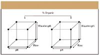
Figure 1: Full factorial design experiments for four factors: pH, flow rate, wavelength, and percent organic in the mobile phase. Runs are indicted by the dots.

During a robustness study, method parameters are varied intentionally to see if the method results are affected. The key word in the definition is deliberate. In liquid chromatography (LC), examples of typical variations are

• mobile phase composition;

• number, type, and proportion of organic solvents;

• buffer composition and concentration;

• pH of the mobile phase;

• different columns lots;

• temperature;

• flow rate;

• wavelength;

• gradient variations;

• hold times;

• slope; and

• length.

Robustness studies also are used to establish system suitability parameters to make sure the validity of the entire system (including both the instrument and the method) is maintained throughout implementation and use.

What is the bottom line? The terms robustness and ruggedness refer to separate and distinct measurable characteristics; or as some refer to it, parameters external (ruggedness) or internal (robustness) to the method. A rule of thumb: if it is written into the method (for example, 30 °C, 1.0 mL/min, 254 nm), it is a robustness issue. If it is not specified in the method (for example, you would never specify: Steve runs the method on Tuesdays on instrument six), it is a ruggedness–intermediate precision issue. In addition, it is a good idea to always evaluate the external ruggedness–intermediate precision parameters separate from the internal robustness parameters.

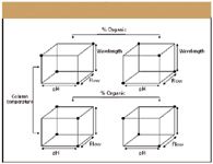
Figure 2: Fractional factorial design robustness study for a five-factor experiment: pH, flow rate, wavelength, percent organic, and temperature. Runs are indicted by the dots.

Robustness Study Experimental Design

For years, analysts have conducted both optimization and robustness studies according to a univariate approach; changing a single variable or factor at a time. Performing experiments in this manner most likely resulted from being trained as scientists (one variable at a time!) as opposed to a statistician. This approach, while certainly informative, can be time consuming, and often, important interactions between variables such as pH changes with temperature remain undetected. Multivariate approaches allow the effects of multiple variables on a process to be studied simultaneously.

Table I: Plackett–Burman design in 12 runs for up to 11 factors. High (1) and low (-1) values correspond to chromatographic variables or factors.

In a multivariate experiment, varying parameters simultaneously, rather than one at a time, can be more efficient and can allow the effects between parameters to be observed.

There are four common types of multivariate experimental design approaches:

• Comparative, used to choose between different alternatives.

• Response surface modeling, used to hit a target, minimize or maximize a response.

• Regression modeling, used to quantify dependence of response variables on process inputs.

• Screening, used to identify which factors are important or significant.

The choice of which design to use depends upon the objective and the number of parameters, referred to as factors, that need to be investigated. For chromatographic studies, the two most common designs are response surface modeling and screening. Response surface modeling commonly is used for method development, but the focus of the remainder of this column will be on screening, because it is the most appropriate design for robustness studies. The references include more detail beyond what is presented here, and additional information on various experimental designs (4–7).

Screening Designs

Screening designs are an efficient way to identify the critical factors that affect robustness and are useful for the larger numbers of factors often encountered in a chromatographic method. There are three common types of screening experimental designs that can be used: full factorial, fractional factorial, and Plackett–Burman designs.

Full Factorial Designs

In a full factorial experiment, all possible combinations of factors are measured. Each experimental condition is called a "run," and the results are called "observations." The experimental design consists of the entire set of runs. A common full factorial design is one with all factors set at two levels each, a high and low value. If there are k factors, each at two levels, a full factorial design then has 2^k runs. In other words, using four factors, there would be 2⁴ or 16 design points or runs. To further illustrate the point, Figure 1 illustrates a full factorial design robustness study for four factors; pH, flow, wavelength, and percent organic in the mobile phase.

Fractional Factorial Deigns

Full factorial design runs can really start to add up when investigating large number of factors; for nine factors, 512 runs would be needed! (Without even taking into account replicate injections.) In addition, the design presented in Figure 1 assumes linear responses between factors, but in many cases, curvature is possible, necessitating center point runs, further increasing the number of runs. For this reason, full factorial designs usually are not recommended for more than five factors to minimize time and expense.

Table II: Example robustness factor selection and limits for an isocratic method. These limits are examples only and should be chosen according to expected laboratory and instrument variations.

So, what do you do if you want to investigate more factors, with or without center points? A carefully chosen fraction or subset of the factor combinations might be all that is necessary, which is referred to as fractional factorial designs. In general, a "degree of fractionation (2^-p )," such as 1/2, 1/4, and so forth of the runs called for in the full factorial design are chosen, as shown in Figure 2. In the previous example, with nine factors resulting in 512 runs for a full factorial design, fractional factorial designs can accomplish the same evaluation in as little as 32 runs (using a 1/16 fraction: 512/16, or 2^k-p . The latter is arrived at by taking the full factorial 2^k * 2^-p or 2^k-p ).

Fractional factorial design works mostly due to the "scarcity of effects principle" that states that while there can be many factors, few can actually be important, and experiments are usually dominated by main effects; not every variable interacts with every other variable. Therefore, the most critical issue in fractional factorial design is selection of the proper fraction of the full factorial to study. There is, of course, a price to be paid for reducing the number of runs and that is that not all factors can be determined "free and clear," but are aliased or confounded with other factors, and the design resolution refers to the degree of confounding. Full factorial designs have no confounding, and have a resolution of infinity. Fractional factorial designs can be resolution 3 (some main effects confounded with some two-level interactions), resolution 4 (some main effects confounded with three level interactions), and resolution 5 (some main effects are confounded with four-level interactions). In general, the resolution of a design is one more than the smallest order interaction that a main effect is confounded (aliased) with. Where possible, important factors should not be aliased with each other. Chromatographic knowledge and the lessons learned during method development (for example, what affects the separation the most?) are very important for selecting the proper factors and fraction. But do not worry, runs can always be added to fractional factorial studies if ambiguities result.

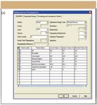
Figure 3(a): Example experimental conditions that might be used for a Plackett–Burman design for an eight-factor ultra performance LC experiment. Shown are the experimental design setup with the factor names and nominal, upper, and lower values.

Plackett–Burman Designs

For robustness testing, it usually is sufficient to determine whether a method is robust to many changes, rather than to determine the value of each individual effect, and Plackett–Burman designs are very efficient screening designs where only main effects are of interest. Plackett and Burman published their now famous paper back in 1946 describing their economical experimental designs in multiples of four rather than a power of two (9), and Plackett–Burman designs frequently have been reported in the literature for chromatographic robustness studies (see, for example, references 10–12). Table I shows a generic Plackett–Burman design for the 12 runs needed to evaluate 11 factors, according to the general formula N – 1 factors. Figures 3a and 3b illustrate an example of some actual experimental conditions that might be used for a Plackett–Burman design for an eight-factor ultra performance LC experiment. A Plackett–Burman design is a type of resolution 3 two-level fractional factorial design where main effects are aliased with two-way interactions. Plackett–Burman designs also exist for 20 (19 factors), 24 (23 factors), and 28 (27 factors) run designs, but these are seldom used in chromatography as there is rarely the need to evaluate so many factors. In instances where N – 1 factors do not result in a multiple of four, "dummy" factors are used.

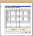
Figure 3(b): Example experimental conditions that might be used for a Plackett–Burman design for an eight-factor ultra performance LC experiment. Shown are the suggested experimental design and conditions for the 12 chromatographic runs.

Determining the Factors, Measuring the Results

A typical LC method consists of many different parameters that can affect the results. Various instrument, mobile phase, and even sample parameters must be taken into account. Even the type of method (isocratic versus gradient) can dictate numbers and importance of various factors.

Typically factors are chosen symmetrically around a nominal value, or the value specified in the method, forming an interval that slightly exceeds the variations that can be expected when the method is implemented or transferred (13–15). For example, if the method calls for premixing a mobile phase of 60% methanol, then the high (1) and low (–1) factors might be 58% and 62% methanol, or some similar range expected to bracket the variability a properly trained analyst using proper laboratory apparatus can be expected to measure. In the case of instrument settings, manufacturers' specifications can be used to determine variability. If the instrument is being used to generate the mobile phase, gradients, or set the temperature, for example, then the range should bracket those specifications. Ultimately, the range evaluated should not be selected to be so wide that the robustness test will purposely fail, but to represent the type of variability routine encountered in the laboratory.

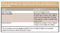
Table III: Example robustness factor selection and limits for a gradient method. Factors and limits listed here are in addition to many of the factors considered in an isocratic method.

Table II lists some factor limits for an isocratic method in which the mobile phase is premixed. Mobile phase composition, flow rate, temperature, and wavelength all are considered. Gradient method factor limits are listed in Table III. Gradient methods represent a slightly different factor selection challenge; in addition to some of the factors that need to be considered for an isocratic method, gradient timing should be taken into consideration.

For any chromatographic run, there are a myriad of results generated. Typical results investigated for robustness studies include critical pair resolution, efficiency (N), retention time of the main components, tailing factor, area, height, and quantitative results like amounts. Note that there are different ways of measuring some of these factors; standard operating procedures (SOPs) or other documentation should specify how the results were calculated. If a quantitative result is desired, it is necessary to measure both samples and standards. Replication of the design points also can improve the estimate of the effects. In addition, it is a good idea to measure results for multiple peaks, as compounds will respond differently according to their own physicochemical characteristics; for example, ionizable and neutral compounds might be present in the same mixture.

Figure 4: Example probability plot. In this example the factor effects are plotted against a linear distribution; departures from the line would indicate robustness issues.

Analyzing the Results

Once the design has been chosen, the factors and limits determined, and the chromatographic results generated, the real work starts. All of that data must be analyzed, and at this point, many analytical chemists begin to search out their resident statistician. Ultimately, the limits uncovered by the robustness study, determined in the data treatment or observed in the graphs, are used to set system suitability specifications.

While consulting and collaborating with a good statistician for robustness studies is always a good idea, there are many tools available to assist the analyst in analyzing the results.

Statistical software is available from a variety of sources. There are add-in programs for Excel, and popular commercially available software such as SPSS (Chicago, Illinois, or spss.com) JMP (Cary, North Carolina, or JMP.com) or Minitab (State College, Pennsylvania, or minitab.com). Third-party software adds to the validation process, as it too needs to be validated.

Chromatography data systems (CDS) also are available that perform many of the requisite calculations and reporting for robustness studies (16). But unlike third-party software, CDSs have the advantage that the data are traceable, validation need only be performed once, and the entire audit trail, relational database, and reporting features can be used not just to generate the data, but also to analyze and report the data during method validation.

Figure 5: Example effects plot. Factor effects can be either positive or negative. The magnitude and direction of the bar indicates the magnitude of the effect.

While a comprehensive statistical discussion is outside the scope of this column, several good references are available for more detail (5–7). A wealth of information also can be found on the internet simply by "Googling" the term of interest or for statistic information in general.

Essentially, the analyst must compare the design results, or the results obtained from the experiments run, for example, according to Table I, or Figure 3, to the nominal results. Regression analysis and calculation of standard or relative error are common ways to look at the data. Analysis of variance (ANOVA), which is a test that measures the difference between the means of groups of data, is another common way of making the comparison. Sometimes called an F-test, ANOVA is closely related to the t-test. The major difference is that, where the t-test measures the difference between the means of two groups, an ANOVA tests the difference between the means of two or more groups.

The primary goal of any robustness study is to identify the key variables or factors that influence the result or response, and graphs are an easy way to observe the effects at a glance. Effects plots and probability plots, are two common ways to represent robustness data, and most general-purpose statistical software programs can be used to generate these plots. As illustrated in Figure 4, in a probability plot the data are plotted in such a way that the points should approximately form a straight line. Departures from the straight line indicate deviations in the data that affect robustness. Different types of probability plots, called normal or half-normal probability plots, are used to further qualify the data. Normal probability plots are used to assess whether or not the data set is approximately normally distributed. Half-normal probability plots can identify the important factors and interactions.

An effects plot is another type of graphical representation, as depicted in Figure 5. Similar to a bar chart, or histogram, the effects plot also can identify the important factors and interactions.

Documentation and Reporting

As the saying goes, if it is not written down, or documented in a report, it is like it never happened. Proper documentation of the robustness study is of course essential to the method validation process. A properly constructed report must include the experimental design used for the study, all of the graphs used to evaluate the data, and tables of information including the factors evaluated and the levels, and the statistical analysis of the responses. The factor limits, and any system suitability specifications arrived at also should be tabulated. A precautionary statement also should be included for any analytical conditions that must be suitably controlled for measurements that are susceptible to variations in the procedure.

Conclusion

A properly designed, executed, and evaluated robustness study is a critical component of any method validation protocol. In a development laboratory, a robustness study can provide valuable information about the quality and reliability of the method, and is an indication of how good a job was done in developing and optimizing the method, indicating whether or not further development or optimization is necessary. When performed early in the validation process, a robustness study can provide feedback on what parameters can affect the method if not properly controlled, and help in setting system suitability parameters for when the method is implemented. Indeed, as recommended earlier, performing the robustness study before evaluating additional method validation parameters can save a lot of time and effort, perhaps preventing the necessity to revalidate.

Acknowledgments

The authors would like to acknowledge the contributions of Jim Morgado (Pfizer, Groton, Connecticut) and Lauren Wood (Waters Corporation, Milford, Massachusetts) for contributions to this manuscript.

Michael E. Swartz "Validation Viewpoint" Co-Editor Michael E. Swartz is a Principal Scientist at Waters Corp., Milford, Massachusetts, and a member of LCGC's editorial advisory board.

Ira S. Krull "Validation Viewpoint" Co-Editor Ira S. Krull is an Associate Professor of chemistry at Northeastern University, Boston, Massachusetts, and a member of LCGC's editorial advisory board..

References

(1) USP 29, Chapter 1225, 3050–3053 (2006).

(2) Int. Conf. Harmonization, Harmonized Tripartite Guideline, Validation of Analytical Procedures, Text and Methodology, Q2(R1), November 2005.

(3) Pharmacopeial Forum 31(2) Mar.-Apr., 549 (2005).

(4) G.E.P. Box, W.G. Hunter, and J.S. Hunter, Statistics for Experimenters (John Wiley and Sons, New York, 1978).

(5) J.C. Miller and J.N. Miller, Statistics for Analytical Chemistry (Ellis Horwood Publishers, Chichester, UK, 1986).

(6) NIST/SEMATECH e-Handbook of Statistical Methods, http://www.itl.nist.gov/div898/handbook

(7) P.C. Meier and R.E. Zund, Statistical Methods in Analytical Chemistry (John Wiley and Sons, New York, 1993).

(8) R.L. Plackett and J.P. Burman, Biometrika 33, 305 (1946).

(9) R. Ragonese, M. Mulholland, and J. Kalman, J. Chromatogr. A 870, 45 (2000).

(10) A.N.M. Nguyet, L. Tallieu, J. Plaizier-Vercammen, D.L. Massart, and Y.V. Heyden, J. Pharm. Biomed. Analysis 21, 1–19 (2003).

(11) S-W. Sun and H-T. Su, J. Pharm. Biomed.Analysis 29, 881–894 (2002).

(12) Y.V. Heyden, A. Nijhuis, B.G.M. Smeyers-Verbek, and D.L. Massart, J. Pharm. Biomed. Analysis 24, 723–753 (2001).

(13) Y.V. Heyden, F. Questier, and D.L. Massart, J. Pharm. Biomed. Analysis 18, 43–56 (1998).

(14) F. Questier, Y.V. Heyden, and D.L. Massart, J. Pharm. Biomed. Analysis 18, 287–303 (1998).

(15) P. Lukalay, and J. Morgado, LCGC 24(2), 150–156 (2006).