Can We Trust Experimental Standard Deviations?

The statistical nature of experiments means that the standard deviation (SD) of replicate analyses is not a constant but a number with some variability: a standard deviation has its own standard deviation. Consequently, a SD calculated from three experiments only is not rugged and even SDs from ten experiments show a great variability. Analysts should be aware that SDs with low scatter are only obtained if 100 or more experiments are performed.

It is common practice to analyse a specific sample several times and to calculate the standard deviation of the results, often added with a ± sign. This figure of merit can also be expressed as the relative standard deviation (RSD) or coefficient of variation (CV) which is a dimensionless number or, after multiplication with 100, in %. For example, the result of a certain analysis is 36 µg/L ± 2.8 µg/L. Presented as a relative value, the RSD is 0.078 or 7.8%. It suggests that we can judge the quality of the analysis somehow. But is this ± 2.8 µg/L carved in stone?

In many real-life situations, it is not possible to check the reliability of a standard deviation because of a lack of time. In this article, experimental HPLC results and computer "experiments" with random numbers are presented which throw some light on the results that are often regarded as "carved in stone".

Experimental for 200 HPLC Experiments

A trivial mixture of four analytes was used for the study of standard deviation (SD) variability: methyl-, ethyl-, propyl- and butylparaben dissolved in the mobile phase at two different concentration levels: 1 mg/L and 0.1 mg/L each. These concentrations represent neither trace analysis nor mass overload conditions on the column. 10 × 10 consecutive analyses of any concentration sample were performed on 10 different days, i.e. ten runs for each day, giving a total of 200 injections. The SDs of the peak areas were calculated for each analyte for each day, i.e. from data sets with number of experiments n = 10.

The experimental conditions were as follows: Instrument: SpectraPhysics with SpectraSystem P4000 pump and low-pressure gradient mixer, a SpectraSystem AS3000 autosampler with 100 µL loop and a SpectraFocus UV detector 254 nm (Spectra-Physics Analytical, Fremont, California, USA). Stationary phase and column: Nucleosil 100 C18 5 µm, 125 × 3 mm (Machery-Nagel AG, Oensingen, Switzerland). Mobile phase: water/acetonitrile (65/35 V/V), 1 mL/min. 20 µL of sample solution were injected. The temperature was ambient.

"Experiments" with Random Numbers

It is possible to generate normally distributed random numbers by Excel: Data > Data Analysis > Random Number Generation. Select "Normal" under Distribution. It is important not to set a value at "Random Seed" but to leave this box empty. By doing so, the generated data are different with every "experiment" but they fulfil the conditions selected for the mean and SD. If a value is set in the "Random Seed" box, the data will always be the same (the procedure is deterministic). However, the numbers generated with or without seed are pseudo-random because Excel uses a certain algorithm.

True random numbers with preselected mean and SD can be generated with www.random.org/gaussian-distributions, a website which is self-explanatory and very easy to use. Its randomness comes from atmospheric noise — a process which cannot be influenced by any means. The generated data can then be transferred into an Excel sheet for further analysis; after the import they are "text" but can be converted to numbers with the data processing options.

Standard Deviations Found with HPLC

Replicate analyses always yield differing results if the number of digits is high enough. Concerning the peak areas obtained with replicate HPLC experiments, their scatter comes mainly from variations of the injection process and from fluctuations of the mobile phase flow-rate if the same sample is analysed. Other possible short-time variations (temperature changes, lamp fluctuations) are usually less important (1), and the same is true for baseline noise if the signal-to-noise ratio (S/N) is high. The day-to-day variations are higher because the composition of the mobile phase could be slightly different, the column has lost a little bit of its performance, the lamp is one day older, etc. This is the reason why it is necessary to set up a new calibration curve every day if quantitative data are needed. Consequently, SDs calculated from the results generated over a longer time span reflect the time-different intermediate precision of the laboratory's performance. But what we are discussing here is the repeatability of consecutive HPLC experiments under the conditions mentioned above.

Table 1: Daily standard deviations of the peak area and their variability of two analytes of different concentration. Ten consecutive experiments for each day. SD = standard deviation, RSD = relative standard deviation.

Naïve thinking may lead to the idea that the SD, obtained with, for example, ten analyses for each day, is a number which can be repeated easily from day to day because the short-term variations will be very similar (as long as the instrument is maintained well, although its performance will decrease over months until the next service is done — but the topic of this paper is not month to month variations).

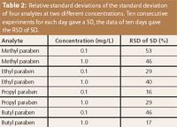
A typical set of experimental data is presented in Table 1: Daily means and SDs from ten consecutive injections per day for ethyl paraben at a concentration of 1 mg/L and of propyl paraben at 0.1 mg/L. The RSDs of the SD are 40% and 16%, respectively. The data of all 200 experiments are summarized in Table 2. They do not show a dependence on the concentration.

Table 2: Relative standard deviations of the standard deviation of four analytes at two different concentrations. Ten consecutive experiments for each day gave a SD, the data of ten days gave the RSD of SD.

It is clear that the SD data represent the actual performance of the instrument. They might be better or worse if obtained with another system. But there are good reasons to assume that the RSD of the SD would look similar in another laboratory with another instrument. The reasons come from computer "experiments" presented in the next paragraph, and they show that ten analyses cannot yield a rugged SD.

Standard Deviations Found with Random Numbers

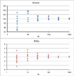
The website www.random.org/gaussian-distributions was used for the generation of data sets of 10 × 3, 10 × 10, 10 × 30, 10 × 100, 10 × 300, and 10 × 1000 random numbers. The means, SDs and RSDs of the SD are shown in Table 3. The means and SDs are also presented in Figure 1.

Figure 1: Means (expected value = 100) and relative standard deviations (expected valule = 3.0) of random numbers with Gaussian distribution. The x-axis represents the number of "experiments" n, namely 3, 10, 30, 100, 300 or 1000. 10 data sets for each value of n were obtained, they are all shown.

It is obvious that three experiments do not yield a rugged SD but a number of high variability, in this very data set with 39% RSD of the SD. Other "experiments" with 10 x 3 random numbers gave RSDs of the SD of 73, 30, 37, 56, 61, 56, 58, 59, 62 and 31% in this order. Data obtained with such a low number of analyses should not be used as quality numbers of merit because they are just too coincidental. By increasing the number of repeated experiments to 10, the RSD of the SD is lower, here 23%. A more rugged SD can only be obtained with a very high number of experiments, for example, 100. Table 3 shows that the system seems to become stable from 300 data points on. Here, by chance, the RSD of the SD is a bit worse with data sets of n = 1000 (2.8%) than with n = 300 (2.5%). If the computer experiments are continued, other data will be generated, namely 2.5% for n = 1000 (similar to the former value) and 3.6% for n = 300 (different from the former value), and so on. The curious reader may play himself or herself with the random number generator. Unfortunately, in the laboratory such large data sets cannot be obtained during validation but only in routine analyses of a stable reference material which is investigated over a long period of time.

Table 3: Data obtained with www.random.org/gaussian-distributions. Required mean = 100, required standard deviation = 3.

Would it be a good idea to "pool" low-number replicates? If, for example, there is time for ten analyses, one could perform 5 × 2 trials, calculate five standard deviations from two trials each, and calculate the mean of the five SDs. Computer simulations show that this approach does not make sense. The variability of the standard deviation obtained from 10 experiments is always lower than the mean from 5 × 2 experiments (SD of the SD is between 0.61–0.88 in the first case and between 0.69–0.99 in the second, obtained with 20 different sets of 50 × 10 random numbers).

The Consequence for the Lazy Analyst

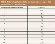
In a normal or Gaussian distribution, the span of ± 1 SD around the mean covers 68.3% of the data whereas 32% lie outside of this range. The span of ± 2 SDs covers 95.4%. Many laboratories follow a "95%" or "2σ" policy although 3σ or even 6σ ("six sigma") gain importance. The expansion from 1 to 2 SDs was investigated by Student in a classical paper (2). Table 4 shows the factors, the so-called coverage factors, which are needed for 95% coverage. This table is the best proof of the fact that three experiments are too low a number with regard to statistics. If one calculated a certain SD from three analyses, it is necessary to multiply the number by 4.3 to reach the 95% coverage! As an example, a 1σ RSD of 3% rises to 13% by expansion to 2σ.

Table 4: Coverage factors (t) for the expansion of a SD or RSD to the 95% confidence interval.

These considerations are equally valid in the field of measurement uncertainty (3). The standard procedure for the evaluation of the measurement uncertainty of an analysis (or another experimental setup) yields the 1σ uncertainty which is then usually expanded to 95% with the appropriate coverage factor. If the laboratory generally works with three replicate analyses which gives the base of the uncertainty evaluation, its performance looks poor after the expansion to the confidence interval of 95% by multiplication with 4.3, the punishment for laziness. It would be much better to invest some time in a larger number of replicates because the effort is rewarded by a lower measurement uncertainty.

The best procedure is the thorough investigation of a reference material based on numerous experiments which results in a statistically sound measurement uncertainty. (Note that no expensive certified reference material is needed for this purpose; a stable and properly stored material, prepared in-house will do the job.) From then on it is even possible to perform single analyses (4) accompanied by the analysis of the reference material. The result of the latter is monitored in a control chart which will show any outliers or long-term trends. If two analyses of the same sample are done (for the calculation of a mean, but not of a SD), they should not be performed simultaneously because the probability is high that the same handling error (in weighing, pipetting, diluting...) will happen at both procedures when working in parallel.

Conclusions

The laws of random are more random in nature than we tend to assume. A SD calculated from three experiments is not a number to be trusted because it has a high degree of randomness. The next three experiments will yield another SD. The data quality of ten experiments is better but even in this case the variability of the SD is astonishingly high. Unfortunately, this is bad news for the analyst. It may even be better to perform a single analysis and to use the repeatability data obtained from the continued investigation of a reference material.

In reports, it must be clearly stated how the SD was determined. Several correct procedures are possible:

• Perform n analyses and note n together with the calculated SD or RSD.

• Perform n analyses and expand to the 95% confidence interval by using the data of Table 4. Note n, the t factor, the expanded SD or RSD and the confidence interval.

Perform one analysis and use the SD or RSD obtained from numerous analyses of a reference material with identical properties as the sample (e.g. an appropriate matrix reference material). Note the details of this approach.

Acknowledgement

Thanks to Dr Bernd Renger, Radolfzell, Germany, for the hint to the generation of normally distributed random numbers by Excel and for the critical review of this paper.

Veronika R. Meyer has a PhD in chemistry. She is a senior scientist at EMPA St. Gallen and a lecturer at the University of Bern, Bern, Switzerland. Her scientific interests lie in chromatography, mainly in HPLC, and chemical metrology such as measurement uncertainty and validation.

References

(1) V.R. Meyer, J. Chromatogr. Sci., 41(8), 439 (2003).

(2) Student (W.S. Gosset), Biometrika, 6(1), 1 (1908).

(3) EURACHEM / CITAC Guide Quantifying Uncertainty in Analytical Measurement, 2nd Edition 2000, ISBN 0-948926-15-5, http://www.eurachem.org/index.php/publications/guides/quam.

(4) A.F. Aubry, R. Noble, M.S. Alasandro and C.M. Riley, J. Pharm. Biomed. Anal., 37(2), 313 (2005).