Selectivity in Reversed-Phase LC Separations, Part II: Solvent-Strength Selectivity

Last month's "LC Troubleshooting" concentrated on solvent-type selectivity (1) — that is, changing the mobile phase solvent in reversed-phase liquid chromatography (LC) separations to change selectivity. Changing solvents is a powerful way to move peaks around in a chromatogram and should not be discounted as a valuable tool for method development. However, you often can get the desired change in selectivity in a simpler way — by changing the solvent strength. When we talk about a strong solvent in reversed-phase separations, we're referring to the organic solvent in the mobile phase — acetonitrile, methanol, or tetrahydrofuran in most cases — usually designated as the B-solvent or %B. Thus, a stronger mobile phase would be one with a higher %B. This month we'll look at the regular changes in retention that are observed with a change in the solvent strength and how to take advantage of them when we develop a method.

John W. Dolan

Retention Factor and Column Dead Time

In many cases with LC separations, it is more useful to deal with the retention factor, k, than with retention time, t_R . The retention factor is calculated easily as

where t₀ is the column dead time. The dead time can be measured by the injection of an unretained substance, observing the rising baseline at the "solvent front," or estimating the column volume, V_m, for 4.6-mm i.d. columns as

where L is the column length in millimeters. So for a 100 mm × 4.6 mm column, the column volume V_m is ≈1 mL. Convert this to t₀ by dividing by the flow rate. At 2 mL/min, we have t₀ ≈ 1 mL/2 mL/min ≈ 0.5 min. We'll use this column and flow rate for the following examples.

Retention Factor and Selectivity

In Figure 1 I've shown simulated chromatograms based on a set of data for a group of nitroaromatic compounds on a 100 mm × 4.6 mm, 3-µm d_p C18 column operated at a 2-mL/min flow rate. In each case, you can spot the t₀ mark at 0.5 min (arrow). We all know from observation that retention time decreases as %B is increased. This is shown with the shorter run times when moving from 55% to 60% to 65% in Figure 1. Another, sometimes overlooked, change is that selectivity, or peak spacing, often changes with a change in %B. For example, in Figure 1 at 55%, peaks 2 and 3 are the closest together. We refer to this as the critical peak pair or, if we are interested in resolution, as the minimum resolution. Note that when the mobile phase is changed to 60%, in addition to the shorter run time, the critical peak pair changes to peaks 4 and 5. A further change to 65% additionally shortens the run and also changes the critical peak pair to peaks 3 and 4. When chromatographic conditions are changed and we observe a change in the critical peak pair, the changed variable is one that can be used to control the separation. In the present example, %B can be used to control the separation. This deserves more study.

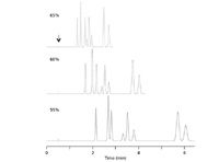
Figure 1: Simulated chromatograms for a mixture of nitroaromatic compounds using conditions listed in text. Arrow indicates t0.

Retention Factor and Solvent Strength

Notice that each peak in Figure 1 moves in a regular fashion as %B is changed. We can observe this more readily if we calculate k for each peak in each run and plot log k against %B, as shown in Figure 2 for peaks 2–5. Two important observations should be made for Figure 2. First, the lines are, for all practical purposes, linear. This means that they can be described by a simple equation:

where k₀ is the k-value at 0% organic, and S is the (negative) slope of the plot. A linear plot means that only two experimental values are needed to calculate k at any %B value. Thus, based on two actual runs, we can predict retention at any other %B value, within the limits of extrapolation from the initial data set, of course.

The second observation from Figure 2 is that, although the slope of the lines for the various analytes are roughly the same, there is enough difference in S that peak spacing changes when %B is changed. On the left edge of Figure 2, it is obvious that peaks 2 and 3 are closest together. This also was observed in the 55% plot of Figure 1. Similarly, at the right edge of Figure 2, it is not quite so obvious, but peaks 3 and 4 are closest together, corresponding to the 65% run of Figure 1. The slopes of the lines for peaks 4 and 5 are very similar, so little change in peak spacing is seen with a change in %B. Peak 3, on the other hand, has a different slope from the other peaks and moves relative to peaks 2 and 4 as %B is changed. Visual extrapolation allows us to predict that peaks 2 and 3 will be coeluted at a mobile phase of <55%, whereas peaks 3 and 4 will be coeluted at some mobile phase > 65%.

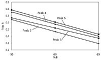
Figure 2: Plot of log k vs. %B for peaks 2–5 of Figure 1.

These two observed behaviors — linearity and a change in relative peak spacing with a change in %B — are what makes solvent strength such a powerful tool for method development. It means that we can leverage a small amount of experimental data to predict the separation under other conditions.

Resolution and Solvent Strength

To take full advantage of solvent strength, we need to make two more calculations, α and N:

where α is the selectivity, or relative peak spacing, for an adjacent pair of peaks with k-values k₁ and k₂.

where N is the column plate number (column efficiency) and w is the peak width measured at baseline between tangents drawn to the sides of the peak.

We can combine k, α, and N to form what is called the fundamental resolution equation:

where R_s is the resolution between two peaks of interest, and k usually refers to the first peak of a peak pair of interest.

Now we have all the information to calculate resolution at any %B for a separation. We first determine the behavior of each peak by making two experimental runs and obtaining the data necessary to calculate k at any %B using equation 3. Now we can determine factor iii of equation 6. If we know k for each peak at any %B, then α for each peak pair can be calculated using equation 4. This gives us data for factor ii of equation 6. All we need to finish the job is to either measure N or for many purposes, an estimate of N is sufficient. A 150-mm column containing 5-µm particles or a 100-mm column filled with 3-µm particles each will generate N ≈ 10,000 for real samples. This is a handy number because (10,000)^0.5 = 100, so now equation 6 simplifies to

which can be used to estimate resolution for any peak pair at any %B based on data from only two experimental runs.

The Resolution Map

Although equation 6 or 7 allows us to calculate resolution for each pair of peaks at various mobile phase strengths, it usually is not the resolution of all peak pairs that we are interested in. We are more interested in the resolution of the critical pair of peaks. If we calculate the resolution between each pair of peaks for a given %B, we can determine which peak pair is the critical peak pair. If we plot the resolution of only the critical peak pair against %B, we get a resolution map, as is shown in the lower part of Figure 3. Chromatograms for peaks 2–5 of Figure 1 are shown for several points on the resolution map (peak intensities slightly different between Figures 1 and 3).

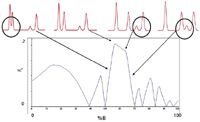
Figure 3: A resolution map for the sample of Figure 1 showing partial chromatograms for peaks 2, 3, 4, and 5. Critical peak pair is circled in each case (peak intensity differs slightly between Figures 1 and 3).

Several powerful aspects of the resolution map should be readily apparent. First, the conditions for the highest resolution are quickly identified: ≈56%. To find this optimum with a search-and-refine optimization process would require many more than two or three runs. For example, an initial run at 90% would give extremely short retention times. A change to 70% would give a chromatogram with k ≈ 1 for the first peak and a run time of about 2 min. Then we might begin refining the conditions 5% at a time until we got close — probably 6–8 runs at a minimum. Instead, we could use the second (70%) run as one of the inputs and then drop %B by 10–15% for a 60% or 55% run. With these three runs (one wasted and two useful), we have sufficient data to generate the resolution map. Finding the conditions for the best resolution is well worth two or three runs.

A second aspect of the resolution map is that we quickly can identify conditions to avoid — in particular those where peak coelution occurs. Coelutions happen whenever the resolution map dips to zero resolution, such as at ≈40%, ≈50%, and ≈70%. At each of these conditions, one or more peak pairs overlap completely. For example, in the right-hand chromatogram at the top of Figure 3, the middle two peaks are seen to be the critical peak pair (circled); as %B is increased, the peaks will move closer together until they are coeluted at 70%, then their resolution will increase as they reverse order and pull apart.

A third important use of the resolution map is to estimate the robustness of the separation to the variable of interest — %B in this case. We can see that the highest resolution is at ≈56% B, but it drops off rapidly as %B is decreased. On the other hand, resolution decreases less rapidly as %B is increased. The relatively flat region of the map between ≈56% and ≈65% will lead us to conclude that if we use 60% as the default mobile phase concentration, the method would be able to tolerate ≈±2% B without major loss in resolution. We could use this information to identify limits to test for robustness testing.

How Good Are the Predictions?

In some ways, the resolution map seems almost too good to be true. Can you really make just two runs and predict retention and resolution at any other %B? Well, yes and no. The "garbage-in-garbage-out" principle holds here — if you gather high quality input data to make the calculations, the results can be quite good. Predictions of k easily have errors of <5% for interpolation between the initial runs and with reasonable extrapolation beyond the input values. Predicted values of resolution are likely to be less accurate due to two factors. One of these has to do with the selection of the plate number used in the calculations. Equation 7 assumes N = 10,000, and it is obviously limited to these conditions. Equation 6 uses a single plate number for all peaks — a generalization that will compromise the predictions, but not too dramatically if the plate number of the peaks of interest is used. The biggest shortcoming of equation 6 is that it does not take peak asymmetry into account. Most peaks tail to some extent, and this tailing tends to reduce resolution. Corrections for tailing are too involved for this limited discussion, but commercial resolution mapping software, such as DryLab (Molnar Institut, Berlin, Germany) can take peak tailing and plate numbers for each peak into account when generating a resolution map, for more accurate results. In any event, the resolution map generated from equations 6 or 7 will identify the conditions for the largest resolution, even if the predicted value of resolution is not exactly what is observed experimentally.

Conclusions

Last month's "LC Troubleshooting" (1) looked at the use of solvent-type selectivity as a means to control the peak spacing in a chromatogram. This month we've looked at the alternative of solvent-strength selectivity. Although solvent-strength changes typically show less-dramatic effects on selectivity than do changes in solvent type, solvent-strength selectivity is powerful enough to identify satisfactory separation conditions in many cases. Because this technique requires only two or three experimental runs, it is easier and faster than changing from one solvent to another. And if %B adjustments alone are insufficient to obtain the desired separation, you have identified conditions for one of the corners of the solvent-selectivity triangle approach discussed last month. For these reasons, I recommend exploring solvent strength before solvent type during method development. Although you can perform all the calculations manually using the equations given here, the process will be much faster and less frustrating if you use commercial resolution modeling software.

References

(1) J.W. Dolan, LCGC North America 28(12), 1022–1027 (2010).