A Quality-by-Design Methodology for Rapid LC Method Development, Part III

Quality-by-design (QbD) is a methodology gaining widespread acceptance in the pharmaceutical industry. A core tenet of this methodology is the idea of establishing the design space of a product or process as a primary R&D goal. Many articles have been published recently describing the successful application of QbD to process development. By recognizing a liquid chromatography (LC) instrument as a small process-in-a-box, one can readily see the applicability of QbD to LC method development.

Michael Swartz

ICH Q8 defines a design space as "The multidimensional combination and interaction of input variables (for example, material attributes) and process parameters that have been demonstrated to provide assurance of quality"(1). Two key elements of this definition warrant brief discussion. First, the phrase "multidimensional combination and interaction" clearly indicates that the "design space" should be characterized by studying input variables and process parameters in combination, and not by a univariate (one-factor-at-a-time) approach. Second, the term "design space" is one of many terms used in the Design of Experiments (DOE) lexicon to denote the geometric space, or region, which can be sampled statistically by a formal experimental design. Other terms in common use include design region, factor space, and "joint factor space."(2). However, the phrase "demonstrated to provide assurance of quality" clearly defines this design space as a subset region of an experimentally explored design region in which performance is acceptable. Therefore, in this article, the term "experimental design region" refers to the geometric region described by the ranges of LC parameters studied in combination by a formal experimental design. When the experimental results are of reasonable quality, DOE can translate the experimental design region into a "knowledge space" within which all important instrument parameters are identified, and their effects on method performance are fully characterized. As DOE is fundamentally a model-building exercise, this translation is accomplished by deriving equations (models) from the experimental results. Given that the equations have sufficient accuracy and precision, they then can be used to directly establish the ICH-defined design space. The instrument parameter settings in the final LC method, thus, represent a point within the design space. The design space itself represents a region surrounding the final method bounded by edges of failure; parameter setting combinations inside the bounds have acceptable method performance, parameter setting combinations outside the bounds do not.

Ira Krull

QbD for Formal Method Development

Many pharmaceutical companies have adopted a two-phased approach to LC method development work in which column–solvent screening experiments are done as Phase 1, followed by formal method development as Phase 2. Part II of this article series described a QbD methodology for Phase 1 in which formal experimental design is used to study column type, organic solvent type, and pH. It also introduced the use of novel Trend Responses to overcome knowledge limitations common to column–solvent screening studies due to the compound coelution and changes in compound elution order across experiment trials (peak exchange). Figure 1 presents a QbD-based workflow proposed for Phase 2 experiments by which an LC process design space can be established. As for the column–solvent screening work, a formal experimental design approach is used in Phase 2.

Defining the experimental design region: The first step in the QbD workflow is defining the experimental region. In LC method development, knowledge of the target compound properties usually determines which instrument parameters are selected for study (Step 1.a). A mistake commonly made in Step 1.b is setting small study ranges analogous to those typically used in method validation for robustness experiments. In such an experiment, each variable's range is normally set to the expected ± 3.0 σ variation limits about its setpoint, as a robustness experiment's purpose is to test the "null" hypothesis — that the factor has no statistically significant effect on method performance across its expected noise range. However, even critical parameters will have inherently small effects across their noise ranges (low signal-to-noise ratio [S/N]), which makes a robustness experimental approach inappropriate to the QbD method development goal of deriving precise and accurate models of study variable effects. Therefore, as a rule of thumb, the experiment variable ranges should be set to a minimum of 10 times their expected noise ranges, and unless restricted by engineering constraints, should never be set to less than five times these ranges.

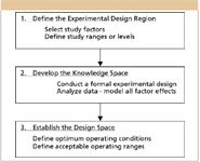
Figure 1: QbD methodology for Phase 2.

Table I presents a template that defines a proposed experimental region for the formal method development phase. As for the Phase 1 template previously presented, this template can be modified as needed to accommodate the specific LC instrument system and compounds that must be resolved.

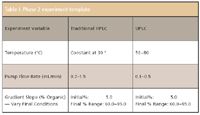
Table I: Phase 2 experiment template

Developing the knowledge space: Step 2 in the QbD Workflow first involves generating and carrying out a statistical experimental design. Selecting the statistical experimental design is a critically important step; there is a wide variety of statistical design types, each of which has specific information properties and is intended to support a specific analysis model. In practical terms, this means that not all statistical designs have the same ability to identify which variables are important and quantify variable effects. Unfortunately, it is observed very commonly that an experimenter will select a design based upon its "size" — the required number of experiment trials for a given number of study variables, and neglect the underlying model form when analyzing the data. A typical example is the widespread use of highly fractionated factorial designs such as the popular Plackett–Burman designs. These designs are two-level fractional factorial designs for studying N —1 variables in N runs, where N is a multiple of four. The simplest case is the N = 4 design for studying three variables at two experimental levels each in four trials. Figure 2 illustrates this design for three variables, designated X1, X2, and X3, at standardized low (—) and high (+) levels. The figure shows the low and high level settings of the three variables in the four trials, and also the derived level settings of the two-way effects terms — obtained by multiplying the level settings of the parent main effects terms in each row. These level settings are used in the data analysis to relate the variable's linear additive (main) effects and two-way (pairwise interaction) effects, respectively, to observed changes in a given result across the experiment trials. A simple examination of the level-setting patterns for these terms reveals the perfect correlation of the interaction terms with the main effects terms across the experiment trials. This correlation pattern is deliberate in Plackett–Burman designs, which are intended primarily for screening large numbers of variables to determine if the variables have any significant effects that warrant further study. Deliberate correlation such as this is termed "effects aliasing." These designs support a linear model, and the aliasing must be considered in the interpretation of results, because it cannot be eliminated by data analysis. This means that any observed effect that the linear model ascribes to, for example, X1, might be due in whole or in part to the aliased X2*X3 term — the interaction of X2 with X3. More experiment trials are required to break the aliasing and make the correct assignments of effects. It should be clear from this discussion that care must be taken when selecting the statistical experiment design, and the information properties of the design must not be forgotten when analyzing data and reporting results.

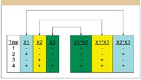
Figure 2: Plackett–Burman design for N = 4.

Careful execution of Steps 1–2.a will correctly stage the experiment to provide the scientific knowledge required to establish accurately the design space for the analytical method in a manner consistent with current ICH guidances: "The information and knowledge gained from pharmaceutical development studies and manufacturing experience provide scientific understanding to support the establishment of the design space, specifications, and manufacturing controls" (1). To illustrate this, we will describe a Phase 2 experiment carried out according to the QbD approach using the sample mix from the Phase 1 "proof-of-technology" experiment described in part two of this article series. The sample mix used in that experiment contained 14 compounds: two active pharmaceutical ingredients (APIs), a minimum of nine impurities that are related structurally to the APIs (same parent ion), two degradants, and one process impurity. The LC instrument platform, which will again be used for this experiment, is a Waters ACQUITY UPLC system (Milford, Massachusetts). Based upon the Phase 1 experiment results, the experimental design region was defined by modifying the Phase 2 experiment template in two ways. First, pH and gradient time were shown to be critical effectors with optimum settings of at 6.8 and 9.5 min, respectively. They were therefore again studied in this experiment to further characterize their effects and establish correct operating ranges. Second, because shallower gradients with high end points were indicated to perform better, the gradient slope was studied by varying the initial conditions with a constant end point. A statistical experimental design was then generated that would support using the full cubic model in the analysis of the results.

Table II: Example Phase II experiment

Once the experiment was run, two unique trend responses described in Part II were derived directly from the chromatogram results (responses). These were: "No. of Peaks" — the number of integrated peaks in each chromatogram, and "No. of Peaks — 1.50 — USP Resolution" — the number of integrated peaks which are baseline resolved in each chromatogram. In addition, peak-result based Trend Responses were used to track the two APIs. Modeling these data facilitated separating them from their respective co-eluting impurities. Trend Response based peak tracking was facilitated by spiking the sample mix such that API 1 was at a significantly higher amount than API 2, which enabled the two related compounds to be distinguished easily in the experiment chromatograms.

Analysis of the experiment data sets yielded a prediction model for each response that identified the important effectors and characterized their effects on the response. Figure 3 illustrates how such a model can be used to predict a response. The figure shows the general form of a partial quadratic model that predicts the resolution of a critical peak pair (Rs) as a function of two experiment parameters, in this case, the pump flow rate (variable X1) and the initial percent organic of the gradient method (variable X2).

Figure 3: Prediction of mean performance.

From Figure 3, one could anticipate that by iteratively entering level-setting combinations of the two study factors and evaluating the predicted results, one could identify the best method obtainable within the variable ranges in terms of the resolution response. One could then plot these iteratively predicted responses in terms of relative acceptability. For example, given a resolution goal of ≥ 1.50, one could generate a modified contour plot of the resolution response in which study factor combinations corresponding to predicted resolution responses below 1.50 are indicated in color, as illustrated in Figure 4.

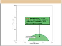
Figure 4: Region of acceptable mean performance.

The dark green line in Figure 4 demarcating the shaded and unshaded regions corresponds to level-setting combinations that are predicted to exactly meet a minimum acceptability value of 1.50 for the critical-pair resolution response within the variable ranges. The demarcation line therefore represents the predicted edge of failure for this response, as defined in the ICH guidance: "The boundary to a variable or parameter, beyond which the relevant quality attributes or specification cannot be met" (3). Taken together, the prediction model (Figure 3) and the corresponding contour plot (Figure 4) numerically and graphically represent the quantitative knowledge space obtained from the DOE experiment for the resolution response.

As discussed in part two of this column series, the models obtained for all responses can be linked to a numerical search algorithm to identify the overall best-performing study variable settings considering all responses simultaneously. In addition, a contour plot like the one in Figure 4 can be generated for each modeled response, and these plots can be overlaid to visualize the global region of acceptability, as illustrated in Figure 5. However, the region of acceptability is consistent with the ICH definition of a design space from a mean performance perspective only.

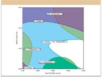
Figure 5: Global region of acceptability.

Establishing the design space: It must be understood that each model derived from the experiment results is a single point predictor of a mean response given the input of a level setting for each study factor (that is, a candidate method). In other words, for a given candidate method, the model predicts the mean (arithmetic average) of the individual resolution values that would be obtained over many injections. The model does not predict the magnitude of the variation in the injections directly, and so cannot provide any knowledge of the relative robustness of the candidate method directly. The region of acceptability illustrated in Figure 5 is therefore only consistent with the ICH definition of a design space from a mean performance perspective. Because method performance varies, methods at or near the edge of failure will only perform acceptably on average. This means that the edges of failure must be moved inside the mean performance design space to accommodate robustness. This "reduced" design space has been referred to as the "process operating space" (3). The question is then how far inside the mean performance design space should the edges of failure be located. Moving them in too far can be overly restrictive and require a level of control that is too costly or unavailable, while not moving them in far enough increases the risk of unacceptable performance. The next section describes in detail how to determine the optimum method and the final design space in terms of both mean performance and robustness without the need to conduct additional experiments.

Characterizing Method Robustness

Integrating quantitative robustness metrics into LC method development is critically important for the simple reason that two candidate methods can provide the same mean performance but very different robustness. This is illustrated in Figure 6 for two methods designated A and B. Both methods have the same mean performance, meaning that on repeated use, they have the same average ability to separate a critical compound pair. But method A performance varies excessively in response to inherent variation in critical LC instrument parameters, while method B performance does not. Unfortunately, it is not possible to determine the relative robustness of a given candidate method by inspecting a resulting chromatogram, and so by simple inspection method A could be identified easily as an acceptable method.

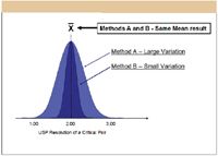
Figure 6: Mean performance versus robustness.

The lack of accurately characterizing robustness in method development is a common reason why many methods must be redeveloped each time they are to be transferred downstream in the drug development pipeline to meet the stricter performance requirements that will be imposed on them. The statements reproduced in the following express how important this integration is in the view of the FDA and the ICH. Although the goal is stated clearly, the guidances do not define how to accomplish such a task. The new methodology presented in this article has been developed in response to both the stated need for integrating robustness into LC method development work and the lack of a defined "how to" approach.

FDA Reviewer Guidance (5). Comments and Conclusions HPL Chromatographic Methods for Drug Substance and Drug Product: Methods should not be validated as a one-time situation, but methods should be validated and designed by the developer or user to ensure ruggedness or robustness throughout the life of the method.

ICH Q2B (6). X. Robustness (8)

The evaluation of robustness should be considered during the development phase and depends upon the type of procedure under study. It should show the reliability of an analysis with respect to deliberate variations in method parameters.

To meet the needs of a working analytical laboratory the new methodology was required to meet three important requirements:

• Be based upon statistically rigorous QbD principles.

• Integrate quantitative robustness metrics without additional experiments.

• Maximize the use of automation to reduce time, effort, and error.

In meeting these three requirements, the new methodology represents the automation of a best-practices approach in which LC methods can be developed rapidly and simultaneously optimized for mean chromatographic performance and method robustness. This new methodology employs Monte Carlo simulation, a computational technique by which mean performance models are used to obtain predictions of performance variation. A detailed description of Monte Carlo simulation is beyond the scope of this paper. For purposes of illustration, the technique is outlined in the following five basic execution steps and illustrated in Figure 7 for the two study factors previously discussed. It is important to note that this approach correctly represents a study factor's variation as random, normally distributed setpoint error, and that the entire error distribution of each factor is represented simultaneously in the robustness computation.

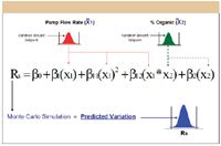
Figure 7: Prediction of performance variation.

A setpoint variation distribution is generated for each study factor using a normal (Gaussian) distribution template with ±3.0 σ limits set to the ±3.0 σ variation limits expected for the factor in normal use. For example, a given target LC system might have expected ±3.0 σ variation limits of ±2.0% about the endpoint percent organic defined in a gradient method.

A candidate method is selected. The method defines the setpoint level setting of each study factor.

For each study factor the setpoint variation distribution is centered at the setpoint level setting, which, thus becomes the effective mean value of the distribution, and a very large number of level settings — say 10,000 — are then obtained by randomly sampling the variation distribution.

The mean performance model then generates 10,000 predicted results — one for each of the 10,000 variation distribution sampling combinations of the study factors. Note that this is a correct propagation of error simulation, because all study factor random variations are propagated simultaneously through the model.

The variation distribution of the 10,000 predicted results is then characterized, and the ±3.0 σ variation limits are determined.

For a given candidate method, the Monte Carlo simulation approach provides a quantitative measure of the variation in a modeled response in the form of predicted ±3.0 σ variation values. This is a good starting point; what is needed then is an independent scale for determining whether the magnitude of the predicted variation is acceptable. For this, we employ the process capability index (C_p) — a Statistical Process Control (SPC) metric widely used to quantify and evaluate process output variation in terms of critical product quality and performance characteristics. C_p is the ratio of the process tolerance to its inherent variation, and is computed as shown in equation 1. Coupling the simulation result with the calculated C_p enables a direct comparison of the relative robustness performance of alternative methods (7).

Note that tolerance limits can be used in equation 1 rather than the more traditional specification limits, because there might or might not be absolute specifications for acceptable variation in critical method performance attributes such as resolution to which this calculation will be applied.

In equation 1, USL and LSL are the upper and lower specification limits for a given response, and the 6σ variation is the amount of the total variation about the mean result bounded by the ±3 σ variation limits. C_p is therefore a scaled measure of inherent process variation relative to the tolerance width. Figure 8 illustrates the C_p calculation elements for the critical pair resolution response described previously given a mean resolution (X) of 2.00 and specification limits of ±0.50. In classical SPC, a process is deemed capable when its measured C_p is ≥1.33. The value of 1.33 means that the inherent process variation, as defined by the 6σ interval limits, is equal to 75% of the specification limits (4/3 = 1.33). Conversely, a process is deemed not capable when its measured C_p is ≤1.00, as the value of 1.00 means that the 6σ interval limits are located at the specification limits.

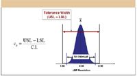
Figure 8: Critical pair resolution response.

The C_p metric can be applied directly to each modeled response to determine the relative robustness of a candidate method in terms of the response and evaluate the robustness on a standardized acceptability scale. However, it is apparent from equation 1 that the C_p value computed for a given candidate method directly depends upon the tolerance limits defined for the response. One should therefore use the following basic rules listed in the following when specifying the specification limits to be used in the C_p calculation.

Specification limits should be defined in the units of the response.

Specification limits should be defined as a symmetrical delta (±Δ) which delineates a relative tolerance range and not as absolute USL and LSL values.

The ±Δ limits will be applied to different candidate methods to determine their relative robustness by computing their C_p values. Absolute USL and LSL values cannot be used, because the mean response will vary across a set of candidate methods being evaluated.

The magnitude of the tolerance limit delta should be consistent with the performance goals defined for the critical response being evaluated.

As an example, a reasonable method development goal is to achieve a mean resolution of ≥2.00 for a critical compound pair. Therefore, an appropriate tolerance limit delta for this response would be ±0.50; this sets the LSL at 1.50, which corresponds to baseline resolution. Note that ever-increasing resolutions usually are not desirable, because as the peaks move farther apart, they also are moving closer to other peaks.

The Monte Carlo simulation approach is used to obtain a robustness C_p value for each method included in the DOE experiment for each modeled response. These robustness C_p results are then modeled as additional response data sets. Recall that the mean performance model of a given result such as resolution represents the combined affects of the study factors on the response within the knowledge space, and predicts the mean result for a given combination of study factor level settings. Likewise, the corresponding robustness C_p model represents the combined affects of the study factors on resolution variation within the knowledge space, and so predicts the resolution variation obtained for a given combination of study factor level settings.

Establishing the Final Design Space

The mean performance and robustness C_p models for the previous ly described responses were linked via numerical optimization routines to identify the study factor level settings that would simultaneously meet mean performance and robustness goals for all responses. The original optimization goals set for the two APIs and their problem impurities were a mean resolution (R_s) of ≥ 2.00 and a Robustness C_p of ≥ 1.33, using tolerance limits of ±0.50 for the resolution robustness C_p calculations. However, the numerical optimization results identified that the best mean performance obtainable within the experimental region was R_s ≥ 1.75 for the APIs with their respective problem impurities, and R_s ≥ 1.50 for one of the problem impurities with its nearest eluted neighbor impurity. Robustness C_p results were therefore re-computed using tighter tolerance limits of ±0.25 and ±0.10, respectively. Table III lists the "best performing method" identified by the automated optimizer relative to the new goals for peak visualization, baseline resolution, and method robustness.

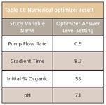
Table III: Numerical optimizer result

Figure 9 illustrates the final design space for pump flow rate and initial % organic (gradient time = 8.3 min, pH = 7.1) as the reduced unshaded region bounded by the new narrower edges of failure required for the responses. Figure 10 is an expanded (zoom in) view of this design space generated by reducing the graphed variable ranges to ranges, which just bracket the new edges of failure.

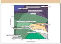
Figure 9: Final design space.

Figure 11 is the chromatogram obtained by analyzing the sample using a method in which the instrument parameters were set to the optimum settings identified by the two experiments. As the figure shows, all compounds are baseline resolved — a result that was not achieved in the prior development effort, which involved more traditional approaches and was underway for over two months. As a final step in this method development effort, the optimized UPLC method was back-calculated to a traditional HPLC method. The back-calculated method met all performance requirements, and was shown to be far superior to the existing QC method, which was developed using a combination of First-Principles and Trial-and-Error approaches. It is especially noteworthy that the combined Phase 1 and Phase 2 experimental work required to obtain this final method consisted of two multi-factor statistically designed experiments, both of which were run on the LC system overnight in a fully automated (walk-away) mode.

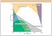
Figure 10: Final design space, expanded view.

Conclusions

As described in Part II of this article series, a Phase 1 column–solvent screening experiment carried out using the new QbD methodology and software capabilities can identify the correct analytical column, pH, and organic solvent type to use in the next phase of method development. These instrument parameters are held constant in the second phase of method development, and the remaining important instrument parameters are then studied, again according to the new QbD methodology, to obtain a method that meets mean performance requirements. However, in LC method development, the commonly used experimental approaches to establishing a design space only address method mean performance — robustness usually is evaluated only separately, as part of the method-validation effort. The novel QbD methodology described here combines design of experiments methods with Monte Carlo simulation to successfully integrate quantitative robustness modeling into LC method development. This combination enables a rapid and efficient QbD approach to method development and optimization consistent with regulatory guidances.

Figure 11: Chromatogram from optimized method.

Acknowledgments

The authors are grateful to David Green, Bucher and Christian, Inc., for providing hardware and expertise in support of the live experimental work presented in this paper. The authors also want to thank Dr. Graham Shelver, Varian, Inc., Dr. Raymond Lau, Wyeth Consumer Healthcare, and Dr. Gary Guo and Mr. Robert Munger, Amgen, Inc. for the experimental work done in their labs which supported refinement of the phase 1 and phase 2 rapid development experiment protocols.

Michael Swartz "Validation Viewpoint"Co-Editor Michael E. Swartz is Research Director at Synomics Pharmaceutical Services, Wareham,Massachusetts, and a member of LCGC's editorial advisory board.

Ira S. Krull

"Validation Viewpoint"Co-Editor Ira S. Krull is an Associate Professor of chemistry at Northeastern University, Boston, Massachusetts, and a member of LCGC's editorial advisory board.

The columnists regret that time constraints

prevent them from responding to individual reader queries. However, readers are welcome to submit specific questions and problems, which the columnists may address in future columns. Direct correspondence about this column to "Validation Viewpoint," LCGC, Woodbridge Corporate Plaza, 485 Route 1 South, Building F, First Floor, Iselin, NJ 08830, e-mail lcgcedit@lcgcmag.com.

References

(1) ICH Q8 — Guidance for Industry, Pharmaceutical Development, May 2006.

(2) D.C. Montgomery, Design and Analysis of Experiments, 5th Edition (John Wiley and Sons, New York, 2001).

(3) ICH Q8(R1) — Pharmaceutical Development Revision 1, November 2007.

(4) A.S. Rathmore, R. Branning, and D. Cecchini, BioPharm Int.20(5), (2007).

(5) FDA — CDER (CMC 3). Reviewer Guidance. Validation of Chromatographic Methods. November, 1994.

(6) ICH-Q2B — Guideline for Industry. Q2B Validation of Analytical Procedures: Methodology. November, 1996.

(7) J.M. Juran, Juran on Quality by Design (Macmillan, Inc., New York, 1992).

(8) R.P. Christian, G. Casella, George, Monte Carlo Statistical Methods: Second Edition (Springer Science+Business Media Inc., New York (2004).

(9) A.J. Cornell, Experiments With Mixtures, 2nd Edition, John Wiley and Sons, New York, 1990).

(10) M.W. Dong, Modern HPLC for Practicing Scientists (John Wiley and Sons, Hoboken, New Jersey, 2006).

(11) R.H. Myers and D.C. Montgomery, Response Surface Methodology (John Wiley and Sons, New York, 1995).

(12) L.R. Snyder, J.J. Kirkland, and J.L. Glajch, Practical HPLC Method Development, 2nd Edition (John Wiley and Sons, New York, 1997).