A Practical Approach to Modelling of Reversed-Phase Liquid Chromatographic Separations: Advantages, Principles, and Possible Pitfalls

Patrik Petersson¹, Bernard O. Boateng², Jennifer K. Field², and Melvin R. Euerby^2,3, ¹Novo Nordisk A/S, Måløv, Denmark, ²Strathclyde Institute of Pharmacy and Biomedical Sciences, University of Strathclyde, Glasgow, United Kingdom, ³Shimadzu UK Limited, Milton Keynes, United Kingdom

Chromatographic principles and best practices for obtaining highly precise retention time, peak width, and resolution predictions for the optimization of reversed-phase liquid chromatography (LC) separations using retention modelling software will be discussed. The importance of fully characterizing the LC instrumentation, how to generate accurate input data, the selection of appropriate models, and peak tracking will be addressed along with a suggested workflow. Adhesion to a few basic rules and simple precautions and the use of modern retention modelling software programmes can assist the rapid development of highly accurate retention models to enable the development of robust and optimized reversed-phase LC separations using either ultrahigh-pressure liquid chromatography (UHPLC) or high performance liquid chromatography (HPLC) conditions. Examples of retention modelling for small and large molecules will be highlighted.

The use of simulation software (1–4) based on chromatographic theory, to predict retention behaviour and to optimize chromatographic separations has now become a pivotal tool in method development strategies for traditional small molecule and the ever-expanding biopharmaceutical drug market (5,6). The main driver for using retention modelling in method development strategies is that it only requires limited input data to rapidly obtain accurate, optimum, and robust separation conditions for the chromatographer’s particular problem.

The prediction accuracy for analyte retention time and resolution is good (6) and the software is flexible enough to allow the chromatographer to model isocratic or gradient separations as a function of variables such as percentage organic, gradient time, gradient shape, pH, temperature, ion-pairing reagent or salt concentration, flow, and column dimensions in a continuous way.

In addition to the one-dimensional modelling described above, two-dimensional modelling-a simultaneous variation of any two-separation variables for a chromatographic procedure-can be accurately modelled. Examples include gradient time versus pH, percentage organic versus pH, gradient time versus temperature, and salt concentration versus temperature (6). Software is also available that can perform three-dimensional modelling (7).

The use of more general optimization software based on entirely empirical models and factorial designs, often referred to as design of experiments (DoE), requires significantly more input data for optimization (8). Another drawback is that it does not simulate the predicted chromatography. This approach requires the definition of one or several response functions to describe the quality of the separation with a single number, a far from trivial task. In our opinion, the most efficient approach is to use retention modelling based on chromatographic theory for optimization and subsequently apply statistical DoE models (that is, reduced factorial designs) for method validation and robustness testing.

Without doubt, the most ubiquitous use of retention modelling is in the reversed-phase liquid chromatography (LC) arena to separate small molecules such as pharmaceutically-active compounds, their synthesis impurities and degradation products, peptide and tryptic digests and protein mixtures, drug metabolites, complex mixtures of active compounds from plant origin, food safety, environmental pollutants, polymer analysis, drugs of abuse, and to estimate the robustness of LC methods (6,9–12). Retention modelling has also been used for translations between ultrahigh-pressure liquid chromatography (UHPLC) to high performance liquid chromatography (HPLC) and vice versa (13), and in Quality by Design (QbD) approaches (14).

Retention modelling is now being successfully applied to characterize proteins, monoclonal antibodies, their charge variants, and antibody–drug conjugates using chromatographic modes such as hydrophobic interaction chromatography (HIC), reversed phase, hydrophilic interaction chromatography (HILIC), and ion-exchange chromatography (IEC) (15–19).

Retention models have also been applied in numerous separation techniques, including gas chromatography (GC) (20), ion-pair chromatography (IPC) (21), HILIC (22), micellar liquid chromatography (MLC) (23), chiral chromatography (24), ion chromatography (IC) (25), and supercritical fluid chromatography (SFC) (9).

This article will describe, in a stepwise manner, how to perform successful and accurate retention modelling using reversed‑phase LC examples and the pitfalls to be avoided to generate accurate predictions. The advice given is equally applicable to all types of retention models and applications using any of the commercial software programmes.

It is hoped that this discussion will encourage and promote chromatographers to adopt this highly accurate and rapid method development tool in their own method development strategies to efficiently generate high-quality LC methods that are fit for purpose.

Experimental

Experimental work was performed on a Nexera X2 UHPLC system (Shimadzu) equipped with LC-30AD pumps, DGU‑20A5R degassers, SIL-30AC autosampler, CTO-20AC column oven, and SPD-M30A photodiode array detector equipped with a 10 μL/10 mm pathlength flow cell, 40 μL mixer (Shimadzu UK Ltd). The system was controlled and data collected by means of LabSolutions software (Shimadzu UK Ltd, version 5.86). A 50 × 4.6 mm, 3-μm ACE SuperC18 column (Advanced Chromatography Technologies Ltd) was used in the study. pH measurements were recorded in the aqueous fraction of the mobile phase. For the dwell volume investigation, a range of differing UHPLC configurations from Shimadzu, Agilent, Waters, and Thermo were evaluated. Modelling was performed using ACD Lab’s LC Simulator (version 2016.2.2).

Results and Discussion

This article will focus on the critically important parameters common to all commercial retention modelling software programmes, characterization of the LC system, and the number and type of input experiments that are required (dependant on the retention model used). Peak tracking and the selection of the most appropriate retention models will also be investigated, all of which are required to generate accurate retention predictions. The generation of suitable samples (for example, forced degradants, mother liquours) will not be covered in this article.

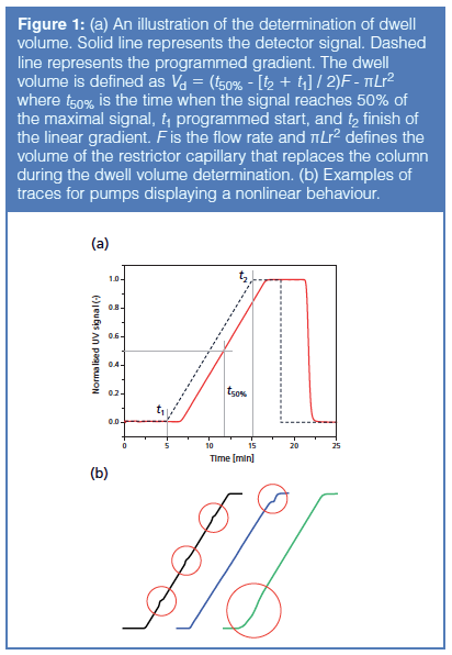
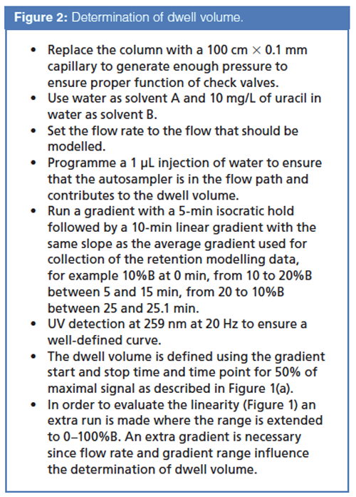
Characterization of the LC System: Most method development strategies, and hence retention modelling, is performed using gradient chromatography, therefore it is vital to establish that the LC system being used is capable of generating a reproducible linear gradient. This can be rapidly established by dwell volume determinations (Figure 1[a] and Figure 2). As can be seen from Figure 1(b), the resultant gradient profile from these three LC systems is unacceptable. If temperature modelling is to be used, the authors recommend that the column compartment should be checked using a calibrated thermocouple and that there is sufficient preheating of the mobile phase before it enters the column, which can be achieved by the use of a preheater or a sufficiently long piece of tubing. The flow rate accuracy must be established at the flow rate of the input experiments (using a flow rate meter or simply from the measurement of the weight of water delivered during a certain time at a certain temperature). The dwell volume should be determined as shown in Figure 2 for the LC configuration that is to be used for the modelling input experiments. The detector sampling rate is not critical for modelling, but it is recommended to record no less than 25 points for each peak so that the resolution is not compromised.

Determination of Dwell Volume:

The dwell volume of an instrument is defined as the volume from the point at which the mobile phases first mix in the pump to the head of the column. The dwell volume can be determined in different ways. In many earlier text books on HPLC and pharmacopoeia publications it was suggested that a wide linear gradient range should be employed, accompanied with a high flow rate (26). However, several instrument manufacturers use a step gradient with a low flow rate and a narrow organic range. We have found that the gradient type (step or linear), flow rate, and gradient range are all critical for the determination of dwell volumes (differences of up to 80% have been observed [27]). We have also found that micro‑fabricated “maze”-type mixers display a larger difference between high and low flow than a traditional type of mixer. Thus, conditions that previously have been suggested for the determination of dwell volumes appear not to be suited for certain UHPLC systems. It is the authors’ opinion that the dwell volume should be determined using gradient conditions that are appropriate for the type of analyte and LC instrumentation that will be used. This will be discussed in more detail in the section called “Gradient Separations”.

Figure 2 describes a procedure that provides an estimate of dwell volumes suitable for modelling purposes. This procedure is based on a linear gradient and it can also be used to ensure that linear gradients can be generated by the system. The procedure displays a good agreement with step gradients at the same flow rate (| ΔVd | <4% 90th percentile for nine UHPLC configurations with dwell volumes ranging from 202 to 718 µL [27]). It also displays a reasonable agreement between measured mixer volumes and nominal volumes specified by the instrument producers ( | Δ mixer volume | <16% for three types of UHPLC systems and nine mixers ranging from 35 µL to 380 µL).

An alternative approach to determine dwell volumes, as well as to compensate for errors in other parameters, is to iteratively try a few different dwell volumes while fitting the model, compare the residuals obtained, and, based on this, select the dwell volume that gives the lowest residual (28).

An error in dwell volume impacts on absolute retention predictions more than relative retention and resolution (29). Fortunately, even a relatively large error in dwell volume of ±20% will only have a small impact on absolute retention; <<1% according to literature (30) as well as our observations (27).

It should be stressed that once a dwell volume has been determined it is not necessary to determine it again unless a significantly different flow rate or gradient slope is used for the generation of models (or the configuration of the system has been changed by an introduction of a larger mixer for example).

Column Dead Volume:

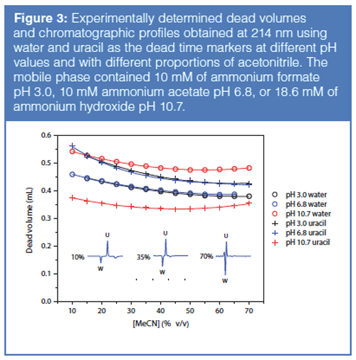
Dead volume is defined as the retention volume for a nonretained analyte. The determination may seem trivial but is actually quite complicated (28). As can be seen in Figure 3, for two frequently used dead volume markers, uracil and water, the value determined depends both on the mobile phase composition and the marker used. At pH 10.7 both water and, even more pronounced, uracil display markedly different dead volumes compared to pH 3 and 6.8. For uracil this is probably a result of repulsion between deprotonated and, therefore, negatively charged uracil (pK_a 8.8) and silanol groups (pK_a range approximately 3.5–6.8 [31]) resulting in a reduced retention. In the case of water, the opposite is observed. This may be a result of water penetrating deeper into the silica surface or pores, which, at pH 10.7, are negatively charged.

Fortunately, it has been found that relatively large errors in dead volume only have a small impact on the quality of predictions. According to previous studies (28–30,32) and our own experience, even an error of ±20% in the dead volume will only result in <1% error in the modelling of isocratic as well as gradient retention.

Uracil is more affected by pH changes than water, and we propose that water should be used as the dead volume marker. At a wavelength of 214 nm water usually produces a well-defined negative peak (Figure 3). For isocratic modelling, we recommend that the dead volume is determined for the average amount of organic modifier used for the generation of the models. For gradient modelling however, we have found that the dead volume for initial gradient conditions gives a better fit than the average dead volume. The determination should be done at the flow rate to be modelled and at the average temperature used during calibration experiments.

Determination of Extra Column Band Broadening (ECBB):

This parameter is a measure of the contribution to peak dispersion that takes place outside the column. Its effect on peak width can become very significant in UHPLC separations. It can be rapidly determined as described in reference 33. In the opinion of the authors, the retention modelling programme should be able to predict the effect of changing this value on the resultant peak width of the analyte. The chromatographer may wish to investigate this if it is necessary to assess the chromatographic performance of a separation when converting from a standard HPLC to a UHPLC configuration (or vice versa).

Selection of Retention Models: The retention models used in today’s optimization software were to a large extent developed during the 1980s by Snyder et al. (34) and Jandera et al. (35). For isocratic reversed-phase LC separations of small molecules, it is often sufficient to use a first order polynomial retention model (equations 1 and 3).

For very high levels of organic modifier where other retention mechanisms come into play, it may be necessary to add a second order term to account for curvature (equation 2). The use of a second order term is also necessary for peptides and proteins where polar and electrostatic interactions are more important and also because their secondary and higher structures may be affected by the organic modifier content and temperature (equations 2 and 4) (36). After optimizing the organic modifier content and temperature for protein separations, it is often advantageous to optimize the trifluoroacetic acid (TFA) concentration. This can be conveniently modelled by a second order model such as equation 2.

The effect of buffer concentration in reversed-phase LC can be modelled using the log–log relationship as described by equation 5. It is possible-but less common-to optimize pH by retention modelling. The reason for this is that the range covered by pH models is often quite narrow compared to the large pH ranges that the chromatographer may wish to exploit. In addition, the prediction errors can be relatively large. pH models typically cover pH ranges close to the pK_a of the analytes of interest and, therefore, big selectivity differences may be observed as the species change their ionization state. The downside to this approach is that peak shape is often poor at a pH close to their pK_a. The robustness and reproducibility are usually poorer because of the high sensitivity of the analyte’s retention to small changes in pH.

Commercial software for retention modelling is based on numerical calculations, and, as mentioned earlier, this allows the combination of models for two variables such as amount of organic modifier and temperature, which has been found to be a very efficient method development strategy (6, 34 p. 92).

[1]

[2]

[3]

[4]

[5]

Where a, m, and q₁ – q₃are analyte and system-specific constants, T is the temperature of the column, Φ the fraction of organic modifier, and C the salt concentration.

Peak width models are based on chromatographic theory (28, 35, 34 p. 378) or, alternatively, on entirely empirical models (22). The latter approach can also be used to model peak asymmetry. How the peak width and peak asymmetry models are defined is usually not visible in the software to the user. The software employed in the current study uses empirical peak width or asymmetry models.

Although it is possible to model the peak asymmetry of the main component, it should be noted that there are no suitable models to adequately describe the shape of the main peak at low level. For this reason, the resolution between a main peak and adjacent impurities are typically poorer than predicted. The workaround is to keep this in mind while locating alternative optimal conditions that give the best possible resolution within an acceptable time and subsequently evaluate these experimentally.

Models are fitted to a calibration data set and the residuals give an assessment of the quality of the model. However, it is good practice to subsequently confirm the model against a validation data set as illustrated in the following examples. As a general rule of thumb, the simplest model should be selected that still gives an acceptable error for the validation data set. A first order model (equation 1) is more robust and allows for more extensive extrapolation than a second order model (equation 2). In order to save time, the collection of a validation data set can be skipped and instead a direct prediction of optimal conditions made based on a first and second order model. Subsequently, both optima are experimentally evaluated and the appropriate model as well as optimal conditions are thereby confirmed.

Input Runs Required for Isocratic and Gradient Modelling: Before attempting retention modelling it is of critical importance to ensure that sound chromatographic conditions are used, for example, by not exceeding the column’s pH and temperature limits. Retention modelling cannot rectify poor chromatographic practice!

Isocratic Separations:

The resolution equation found in any standard chromatographic textbook (equation 6) illustrates that the resolution generally improves with increasing retention for isocratic separations up to a retention factor (k) of approximately 10 (assuming that the selectivity is not affected by changes in conditions). Above k ≈ 10, the retention time increases without any significant gains in resolution. A k <1 normally results in poor resolution and there is also a potential risk from interfering matrix peaks near the void volume. In order to optimize an isocratic separation, it is important to find a good balance between retention time and resolution. Different analytes might respond differently to changes in conditions and thus it is not evident that the longest retention always results in the highest resolution. To identify optimal conditions, it is therefore quite useful to use retention modelling. To obtain good retention models for 1 < k  < 10 it is important to build these models on experimental data determined for k ≈ 3 and ≈ 9 (if a three-parameter model is used also k ≈ 6). An empirical trial-and-error approach can be used to find conditions that provide such k-values. As a rule of thumb, k increases by a factor of three for a 10% reduction in amount of organic modifier (34 p. 237). By having k-values for two or more conditions it is possible to use equation 1 to calculate suitable conditions. In our experience it is more efficient to predict the suitability of isocratic conditions for isocratic modelling based on a simple gradient model (see “Gradient Separations” section).

[6]

Where α is the selectivity factor and N the number of theoretical plates for an isocratic separation.

Gradient Separations:

The resolution equation (equation 7) is also valid for gradient elution chromatography provided that k, α, and N are defined as instantaneous values as the analyte passes the mid-point of the column, k*, α*, and N* (34 p. 39 and p 90).

[7]

Assuming that isocratic retention can be described by equation 1 it is possible to define an expression for which gradient time, t_G, gives a certain retention k*.

[8]

Where V_m is the column dead time, ΔΦ the gradient range, m a parameter in the retention equation (equation 1), and F the flow rate.

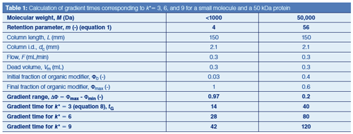
An approximation for the m term can be calculated using the molecular weight (M) of the analyte m ≈ 0.25M0.5 (34 p. 18). Using equation 8 and the m-value approximation it is possible to calculate gradient times that give k*-values which cover the range of interest 1<k*<10 and are therefore suitable for generation of models. As a rule of thumb, gradient times used for calibration should differ by a factor of three (34 p. 92 and p 400). We therefore aim for gradient times corresponding to k* values of 3 and 9. For small molecules it is possible to use a wide gradient range 3–100% acetonitrile (<3% is not recommended for C18 columns because this may result in dewetting of pores previously referred to as phase collapse). Table 1 shows one example of the calculation of gradient times and conditions suitable for a typical UHPLC separation of small molecules. For large molecules, such as peptides and proteins, it is necessary to reduce the gradient range to achieve k* ≈ 3, 6, and 9 within a reasonable time. A typical example for a 50,000 Da protein is also shown in Table 1. A suitable gradient range is defined based on a scouting run, for example 3–100% over 30 min. Based on the retention time of the first peak of interest, it is possible to calculate a suitable initial gradient mobile phase composition using equation 9. It is common practice to subtract a few %B from the initial gradient composition to provide some separation from the early-eluting matrix peaks. The final gradient composition is defined in the same way based on the retention of the last eluting peak of interest. In addition, it is also possible to increase the flow rate if pressure permits and thereby further reduce the gradient times (equation 8). However, keep in mind that this will result in a somewhat reduced resolution because of the steep van Deemter curve displayed by large molecules.

In order to fit models, it is important to ensure that the gradient range is defined so that the analytes elute on the linear part of the gradient that is not in the isocratic dwell volume or at the hold at the end of the gradient. It is also an advantage to keep the buffer concentration the same in mobile phases A and B to reduce superimposed salt and organic modifier gradients, which can be difficult to model (this also minimizes drifting baselines).

When working with peptides and proteins it is common practice to use segmented gradients where a shallow gradient is required to maximize resolution around the main peak. This is bracketed with a steep initial and final gradient in order to capture very hydrophilic and hydrophobic degradation products or process impurities. When generating models, it is usually only this shallow part that is changed to achieve different k*.

[9]

Isocratic or Gradient Separations at Different Temperature:

As previously mentioned, large differences in selectivity can be obtained by simultaneously optimizing the amount of organic modifier and temperature (34 p. 92). In order to fit such models, it is necessary to collect data at different temperatures for each mobile phase composition (or gradient slope). For small molecules it is usually sufficient with two temperatures, for example, 30 °C and 60 °C. However, for peptides and proteins whose secondary structure changes with temperature it is typically necessary to use three temperatures, such as 30 °C, 45 °C, and 60 °C. Thus, these types of modelling require 2 × 2 = 4 or 3 × 3 = 9 experiments.

Collection of Input Data for Fitting of Models: Before retention times are collected for generation of retention models, it is important to ensure that the instrument delivers linear gradients as well as stable retention times. Also, it is often forgotten that a sufficiently long equilibration time should be used so that the column is at a steady state prior to the next gradient. For reversed-phase LC it is typically recommended that at least 10 column volumes should be used (34 p. 170). Once a method has been developed, it is usual to investigate whether the number of column volumes can be reduced (that is, before the retention of early peaks is affected) hence increasing productivity. Other types of chromatography such as HILIC and IEC typically often require > 20 column volumes to establish a steady state. Changing between different %B isocratic conditions in reversed‑phase LC also typically requires equilibrating the column with 10 column volumes.

It should be noted that some proteins may require priming or conditioning of the column with the protein prior to establishing stable retention times; the heat of friction in the column may also require that a couple of “dummy runs” should be performed to obtain a stable column temperature. The same principle must be used when changing other variables such as temperature. The chromatographer must be assured that the system is at a steady state-it is a paradox that rapid and accurate retention modelling cannot be rushed!

It is recommended that the peak width is determined at half height and subsequently the peak width calculated at base line (using equation 10) if that is what is required by the software used for modelling. The reason is that the latter cannot be directly determined for partially coeluting peaks.

[10]

Where w_13.4% is the peak width at baseline (4σ which actually is defined at 13.4%) and w_50% is the peak width at 50% (2.35σ). If a linear gradient is used and peaks are symmetrical it is usually not necessary to determine the width of each peak in the chromatogram. It is then often acceptable to assume that all peaks have a similar peak width and therefore use an average peak width determined for well separated early and late peaks. Isocratic separations require that the width of all peaks be determined because peak width increases with increasing retention. If the chromatograms contain overloaded or asymmetric peaks it is necessary to determine the width of each of these peaks. The width of such peaks is determined at 4.4% (5σ) and then recalculated (equation 11) to 4σ to better reflect the relatively broader peak in the modelling.

[11]

It is also recommended to determine and model the asymmetry of these peaks. It is essential to ensure that the chromatographic data system’s peak asymmetry calculation is the same as the required retention modelling software definition of peak asymmetry.

It is not necessary to determine peak areas to generate models. Peak areas do not affect the resolution or the quality of the separation. Peak areas are only used to facilitate visual comparisons of calculated and experimental chromatograms. Therefore, it is sufficient to determine peak areas for one of the experiments where most of the peaks are well separated and then use these areas as inputs for the other conditions. If peaks are not well separated, areas from different peaks in different experiments can be combined.

To obtain a good agreement between calculated and experimental chromatograms, it is important to use the same equipment, column, and batch of solvents that was used to obtain data for the generation of models. It is also an advantage if the time between building and verification of the models is minimized.

Peak Tracking and Peak Identification: Effective and rapid assignment of peaks in the input chromatograms remains the “Achilles heel” of retention modelling and optimization. If not done properly, incorrect peak assignment will obviously result in incorrect models being developed.

There are many approaches that can be used, from simple manual ones to fully automated techniques. The authors have practical experience of many of these approaches and will briefly describe them and their advantages and disadvantages.

In the development of a LC method, the chromatographer is often faced with several samples from various forced degradation studies of the drug substance, drug formulations, or mother liquors from the drug synthesis, hence, each input run may require results from multiple chromatograms. Therefore, a way is needed to assign the identity of each peak and its origin, before constructing a combined table of peak identities and their origin, retention times, peak widths, peak area, and possibly peak symmetry for each experimental input condition, which can then be entered into the selected retention model.

Peak assignment or identity is best performed by a combination of mass spectrometry (MS), diode-array UV spectra (DAD), or peak area ratios. Occasionally standards of the impurities are available that can be individually chromatographed to aid peak assignment, but this approach can result in more samples being run, extending the sequence duration.

Many of the commercial automated and semi-automated peak‑tracking approaches of software manufacturers do not handle multiple samples because they assume that all components of interest are present in the same sample-in a real‑life situation this is rarely the case. Hence, it is necessary either to perform pooling of samples, which can result in a dilution of the peaks, or to rely on a manual peak tracking approach. It should be stated that retention modelling software requires that there should not be any missing data for any of the analytes that are modelled.

Automated Peak Tracking Software:

Automated peak tracking software based on MS or UV DAD peak-tracking algorithms are available (37,38). The advantages of using automated peak tracking software are reduced operator error, rapid peak assignment, and fully documented method development history. The downside is a significant investment in both software as well as operator skill because the programme is aimed at the experienced chromatographer who performs method development tasks on a routine basis.

Manual Approach:

In laboratories that do not use automated peak tracking software it is still common for chromatographers to literally stick the input chromatograms onto a wall and then, based on a combination of UV DAD spectra, MS and peak area ratio, to manually identify and annotate each peak on the chromatograms. This can be a laborious process but it is still by far the one most favoured by many chromatographers. An Excel spreadsheet is then constructed, which can be copied and pasted directly into the retention modelling software. The advantages of this approach include the low cost and simple implementation, and it does not rely on any peak tracking technique; the obvious disadvantage is that it is time-consuming and prone to operator error.

Examples: Modelling can be used in different ways to assist method development. The most common approach is comprehensive modelling where retention and peak width are modelled for all the peaks of interest. A simpler approach involves only peak tracking and modelling of the main peak along with the first and last peaks of interest. The retention models are then used to define conditions in different parts of the experimental domain that give an acceptable retention and separation window for the modelled peaks. Subsequently these conditions are screened and the one that empirically gives the best separation is selected as optimal conditions.

Conducting a 3 × 3 experiment, which is necessary to construct the models, and then performing peak tracking, affords a better understanding of the separation compared to optimization strategies, which simply screen and count the number of peaks obtained. Peak tracking and modelling also reduces the risk that a peak could move in and out from under the main peak unnoticed. Modelling can be used to locate optimal conditions, to assess and optimize robustness, and facilitate the definition of system suitability tests by the identification of critical peak pairs.

Typical prediction errors have previously been reported to be accurate to | Δt_g | <1% (34 p. 399), | Δw | <17% (28, 34 p. 400), and | ΔR_s | <10% (34 p 119, p. 399). As can be seen in the two examples shown (Tables 2–3) using modern UHPLC instrumentation, prediction errors can be observed that are significantly better. This could possibly be related to a better performance of the latest generation of UHPLC equipment, resulting in better repeatability and reproducibility.

In this article we have defined the prediction error as the 90th percentile for the prediction error, that is | (predicted – actual) | 100/actual. In our opinion, the 90th percentile gives a better idea of what prediction error to expect than the standard deviation, which is sometimes used.

The following sections will describe different types of comprehensive modelling together with some important aspects to consider. We have not included any examples of isocratic to gradient predictions because this is not very useful from a practical point of view.

Gradient to Gradient Prediction Example:

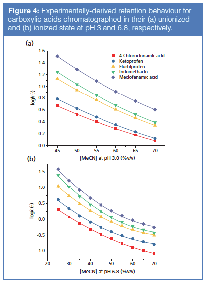
This will be illustrated by the separation of a range of carboxylic acids, including various nonsteroidal anti-inflammatory drugs. Acids are often chromatographed in their ion‑suppressed state at low pH. The reason is that this typically results in enhanced retention, selectivity, and peak shape (at pH 3 logD range of the acids = 2.76–5.92, whereas at pH 6.8 logD = 0.35–3.14). An additional, less well known, advantage that assists modelling is that this results in linear log k versus Φ relationships compared to the nonlinear observed with ionized acids chromatographed at intermediate pH (Figure 4).

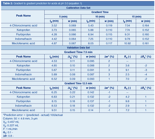
As can be seen in Table 2, linear first order polynomial models provide excellent retention time predictions at pH 3. The employment of a second order model only slightly improves the predictions ( | Δt_g | <0.2% versus <0.1%). It should be stressed that the accuracy of a linear first order model should be evaluated before using a second order model. The reason is that a second order model is less robust (potential for overfitting) and is also less applicable for extrapolation. Consequently, the first order model was selected in this example. Peak width and resolution predictions were also excellent ( | Δw | and | ΔR_s | both <3%). These should not be significantly affected by the selection of retention model.

Gradient to Isocratic Prediction Examples:

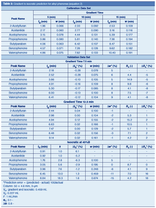
Prediction of isocratic retention based on gradient retention models often results in poorer predictions than gradient to gradient or isocratic to isocratic predictions. Figure 5, which has been constructed from gradient to isocratic predictions of acidic and basic analytes, when chromatographed at different pH, highlights that acceptable retention time predictions are only achievable for retention factors in the range of ~5 to ~25. This can also be seen for isocratic predictions based on gradient models made for alkyl phenones in Table 3 where predictions for 6 <k <18 gave retention time errors of <3% whereas k < 3 gave 5–6% ( | Δw | <13% and | ΔR_s | <17%). The gradient models (three input runs and second order models) used for these isocratic predictions generated gradient retention time errors of only <0.3%.

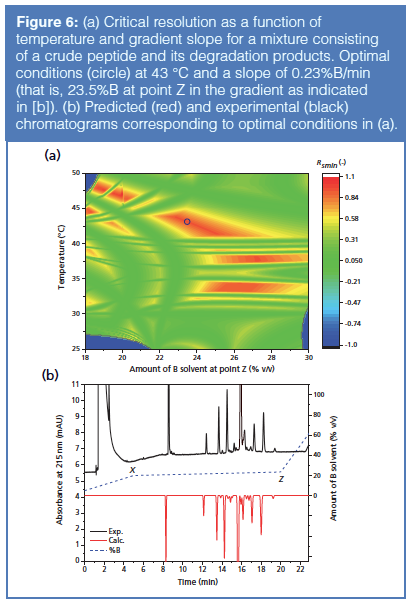
Considering the relatively poor prediction accuracy for gradient to isocratic predictions, we recommend that gradient models be only used to predict approximate isocratic conditions, which can then be used to generate accurate isocratic models (See “Isocratic to Isocratic” section). The separation of peptides and proteins often requires a very shallow, almost isocratic, gradient over the main peak. Consequently, prediction errors for retention often become larger than for gradient to gradient predictions for small molecules. Figure 6(a) shows the resolution map for a mixture consisting of a crude peptide and its degradation products. The predicted and experimental chromatograms corresponding to optimal conditions in the resolution plot are shown in Figure 6(b). The retention time prediction errors in this example were <2% for impurities eluting in the shallow part of the gradient between 10 min and 20 min.

Isocratic to Isocratic Prediction Example:

Isocratic to isocratic predictions are illustrated with the mixed-mode separation of three protonated bases, methoxydiphenidine isomers (MXP), on a reversed-phase material at pH 6.8. As can be seen in Table 4, good predictions can be obtained when applying a second order model and restricting predictions to interpolation ( | ΔtR | <1%, | Δw | <13%, and | ΔRs | <11%). As previously mentioned, the use of extrapolation with second order models is likely to result in poorer predictions, as illustrated in Table 4 with the 35%B validation run where the prediction error for retention increases approximately three times.

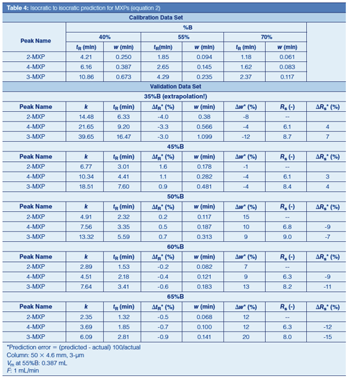
Because of the mixed mode retention at intermediate pH, first order models do not provide acceptable predictions. Models fitted to data at 40, 55, and 70%B result in retention prediction errors of | ΔtR | <9%, which are eight times larger than what was obtained with the second order model (even <19% if extrapolation is made to 35%B).

Although gradient-to-gradient retention prediction accuracy (Δt_g<0.2%) is consistently better than isocratic-to-isocratic (Δt_g<1%), any error of <1% is likely to be of little practical significance. In contrast, gradient-to-isocratic predictions (Δt_g<3–6%) are sufficiently large that this technique is best reserved for initial screening runs only.

Conclusions

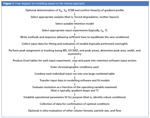
Adhesion to a few basic rules, simple precautions, and the use of modern retention-modelling software programmes can assist the rapid development of highly accurate retention models enabling the creation of robust and optimized reversed‑phase LC separation using either UHPLC or HPLC conditions (Figure 7). The accuracy of the retention, peak width, and resolution predictions today appears to be better than those quoted in earlier papers. This may simply be a result of improved LC systems, more accurate linear gradients, improved chromatographic reproducibility from run to run, and a better understanding of what input runs and models are required.

Acknowledgements

The authors would like to thank Advanced Chromatography Technologies Ltd for supplying the columns used in this work, the Chromatographic Society for support through a summer studentship to B. Boateng, Novo Nordisk for funding J. Field’s PhD studies, and Dr O.B. Sutcliffe (Manchester Metropolitan University, M15GD) for kindly synthesizing and supplying the individual 2-, 3-, and 4-methoxydiphenidine hydrochloride isomers.

References

1. http://www.acdlabs.com/products/com_iden/meth_dev/lc_sim/ (accessed 6/10/2017).

1. http://molnar-institute.com/drylab/ (accessed 6/10/2017).

1. http://www.chromsword.com/products/ (accessed 6/10/2017).

1. http://www.datalys.net/ (accessed 6/10/2017).

1. S. Fekete, R. Kormány, and D. Guillarme, LCGC Special Issue30(6), 14–21 (2017).

1. J.W. Dolan, L.R. Snyder, N.M. Djordjevic, D.W. Hill, D.L. Saunders, L. Van Heukelem, and T.J. Waeghe, J. Chromatogr. A803, 1–31 (1998).

1. M.R. Euerby, G. Schad, H-J. Rieger, and I. Molnár, Chromatography Today, 13–20 (2010).

1. http://www.smatrix.com/fusion_lc_method_dev.html (accessed 6/10/17)

1. D. Spaggiari. V. Desfontaine. A.G-G. Perrenoud, S. Fekete. S. Rudaz. and D. Guillarme, J. Chromatogr. A1371, 244–56 (2014).

1. A. Tölgyesi, R. Berky, K. Békési, S. Fekete, J. Fekete, and V.K. Sharma, J. Liq. Chrom. Rel. Techn. 36, 1105–1125 (2013).

1. R. Kormány, J. Fekete, D. Guillarme, and S. Fekete, J. Pharm. Biomed. Anal.89, 67–75 (2014).

1. R. Hanafi, H. Spahn-Langguth, L. Mahran, O. Heikal, A. Hanafy, H. Rieger, I. Molnár, and H.Y. Aboul-Enein, Chromatographia 79, 469–477 (2012).

1. R. Kormány, I. Molnár, and J. Fekete, J. Pharm. Biomed. Anal. 135, 8–15 (2017).

1. R. Kormány, I. Molnár, and J. Fekete, LCGC North America 32, 354–363 (2014).

1. P. Petersson, J. Munch, M.R. Euerby, A. Vazhentsev, S.K. Bhal, and K. Kassam, Chromatography Today7, 15–18 (2014).

1. E. Tyteca, J.-L. Veuthey, G. Desmet, D. Guillarme, and S. Fekete, Analyst141, 5488–5501 (2016).

1. S. Fekete, J.-L. Veuthey, A. Beck, and D. Guillarme, J. Pharm. Biomed. Anal.130, 3–18 (2016).

1. S. Fekete, S. Rudaz, J. Fekete, and D. Guillarme, J. Pharm. Biomed. Anal.70, 158–168 (2012).

1. S. Fekete, I. Molnár, and D. Guillarme, J. Pharm. Biomed. Anal.137, 60–69 (2017).

1. D.E. Bautz, J.W. Dolan, and L.R. Snyder, J. Chromatogr. 541, 1–21 (1991).

1. R.C. Kong, B. Swachok, and S.N. Deming, J. Chromatogr.199, 307–316 (1980).

1. M.R. Euerby, J. Hulse, P. Petersson, A. Vazhentsev, and K. Kassam, Analytical and Bioanalytical Chemistry407, 9135–9152 (2015).

1. J.R-Montano, C.O-Bolsico, M.J. Ruiz-Angel, and M.C. Garcia-Alvarez-Coque, J. Chromatogr. A1344, 31–41 (2014).

1. R.M. El-Nashar and H.Y. Aboul-enein, Chirality17, 506–513 (2013).

1. I. Molnár, LCGC Europe14(4), 231–237 (2001).

1. Section 2.2.4.6, “Chromatographic Separation Techniques,” European Pharmacopoeia (European Directorate for the Quality of Medicines, Strasbourg, France, 7.0th Ed).

1. M.R. Euerby and P. Petersson, Personal communication/unpublished results (2017).

1. N. Lundell, J. Chromatogr.639, 97–115 (1993).

1. L.R. Snyder and M.A. Quarry, J. Liquid Chromatography 10, 1789–1820 (1987).

1. B.F.D. Ghrist, B.S. Cooperman, and L.R. Snyder, J. Chromatogr. A459, 1–23 (1988).

1. A. Méndez, E. Bosch, M. Rosés, and U.D. Neue, J. Chromatogr. A986, 33–44 (2003).

1. M.A. Quarry, R.L. Grob, and L.R. Snyder, J. Chromatogr.285, 19–51 (1984).

1. https://www.sigmaaldrich.com/content/dam/sigma-aldrich/docs/Supelco/General_Information/t408143.pdf (accessed 6/10/2017).

1. L.R. Snyder and J.W. Dolan, High performance gradient elution: The practical application of the liner-solvent strength model (John Wiley & Sons, Hoboken, New Jersey, USA, 2007).

1. P. Jandera, J. Chromatogr. A1126, 195–218 (2006).

1. M.T.W. Hearn and G. Zhao, Anal. Chem.71, 4874–4885 (1999).

1. G.A. Von Wald and M.T. Vagnini, “Evaluation of ACD/Autochrom Software for LC Method Development,” paper presented at HPLC, San Francisco, California, USA, 2016.

1. K. Jayaraman, A.J. Alexander, Y. Hu, and F.P. Tomasella, Analytica Chimica Acta696, 116–124 (2011).

Melvin Euerby is the Principal of Shimadzu’s Centre of Excellence for Liquid Chromatography and Professor at the University of Strathclyde and the Open University.

Bernard Boateng was a MSc student at the University of Strathclyde and is now a PhD student at the National University of Ireland in Galway.

Jennifer Field is a PhD student at the University of Strathclyde, UK.

Patrik Petersson is a Principal Scientist at Novo Nordisk A/S and Associate Professor at Uppsala University, Sweden.