Optimizing Splitless Injections in Gas Chromatography, Part II: Band Broadening and Focusing Mechanisms

In Part II of our exploration of splitless injection, we will see that it is a surprisingly complex process, and that it is difficult to understand because we cannot see what is happening during the injection process. For this discussion, we will think of the injection process as beginning with the syringe plunger being depressed and ending with the start of a temperature program in the column oven. In most splitless injections, this process requires 30 s to 1 min. There are several band broadening and focusing mechanisms that affect the peak shapes, widths, and heights resulting from splitless injection.

In Part I of this article, we explored reasons why splitless injection is so popular and useful, even though it is complex (1,2). The first minute of a separation involving the splitless injection technique is critical. Figure 1 shows a chart of processes that occur simultaneously during the first minute, and shortly thereafter, in typical split and splitless injections. In the split injection, the purge vent is continuously open, and the column temperature program can start at any time. In the splitless injection, the instrument is set to an initial state of split vent closed, low column oven temperature, high inlet temperature, and carrier gas flow rate appropriate to the method. During the injection period, it does not matter whether the system is in constant pressure or constant flow mode.

FIGURE 1: Flow chart showing temperatures, flows, and valve conditions during (a) split and (b) splitless injection. Reprinted from LCGC North America 2020, 38 (7), 392–395 with permission of the author.

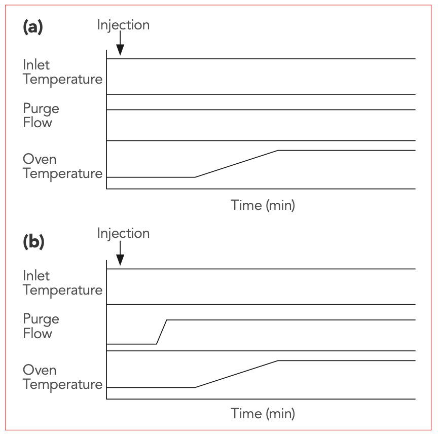
At the instant of injection, the temperature program is started. I recommend that the oven be kept isothermal for the first minute of the separation, or for at least while the split vent is closed, so that only one process, the injection, is happening at the beginning of the run. While the split vent is closed, the injected sample is slowly evaporating in the inlet, its vapor is mixing with the carrier gas, and it is transferred to the column. Within the inlet, two processes are occurring: band broadening in time, and band broadening in space. As the sample vapors reach the cool column, they condense at the column head and are refocused into sharp bands by thermal focusing, solvent effects, or a combination of the two. As seen in Figure 1, a splitless injection is a complex process involving the syringe, the inlet, and the column.

Evaporation in the Syringe

Most chromatographers do not realize that the first place where sample evaporation can occur is in the syringe needle, as the syringe is injected into the hot inlet and the plunger is depressed. In the past, using manual injections, which are often slow and irreproducible due to evaporation in the needle, there were several syringe handling techniques, described using terms such as “hot needle,” “filled needle,” “solvent sandwich,” and the like, used to improve performance. Today, for nearly all injection techniques, including splitless, a fast autosampler is the preferred injection device and speed.

Injection using an autosampler with syringe happens very quickly, with the needle penetrating the septum, the plunger depressed, and the needle retracted within a fraction of a second. The entire sample that leaves the syringe is contained in a solvent band that is therefore a fraction of a second wide, and has little time for evaporation to occur in the needle. We will now discuss how, within the inlet, the band is broadened, and then how, at the column head, it is refocused.

Band Broadening in Time

Band broadening in time occurs because of the splitless injection involving slow carrier gas flow through the inlet. For example, if the volume of the glass inlet liner is 1 mL and the carrier gas flow rate at the column head is 1 mL/min, it will require 1 min for the carrier gas to fully sweep the liner volume, carrying most of the vaporized sample into the column. This contrasts with a split injection, in which the flow through the glass inlet liner is usually very rapid, and sample transfer into the column occurs in a fraction of a second. In a splitless injection, the bands or peaks enter the column with a peak width, measured in time, roughly equivalent to the “purge off” time. When the purge is turned on at the conclusion of the splitless injection, the inlet liner is swept with a very large flow of carrier gas that flows out the split vent, clearing the liner of remaining sample and solvent vapor.

The “purge off” time must be optimized individually for every method involving splitless injection. This is a simple experiment, illustrated in Figure 2. The peak area is plotted against the “purge off” time, which is increased until the peak area is maximized. Note that, like similar curves seen for shaking times in liquid–liquid extraction (LLE) or extraction time in solid-phase microextraction (SPME), it is best to set a “purge off” time on the plateau of the curve. In this example, a 60-s “purge off” time should work well, even though the maximum is first reached in 45 s. While 45 s gave the same peak area as 60 s, it is also close to the region where the curve slopes; minor variation in the “purge off” time or the flow rate might have an impact on the peak area and the reproducibility. Working on the plateau limits this effect.

FIGURE 2: Peak area as a function of “purge off” time.

Band broadening in time is also influenced by sample solvent choice. When a liquid sample is injected, the solvent evaporates; the volume of vapor generated is very dependent on the nature of the solvent, with more polar solvents usually generating much greater vapor volumes. With greater vapor volume, more time will be required for the vapor to be swept from the inlet liner into the column, increasing band broadening in time. To assist in understanding the impact of solvent vapor volume, vapor volume calculators are available online (3,4). Table I shows the vapor volume generated for several solvents, determined using the Restek calculator, with assumed inlet temperature of 250 °C, head pressure 10 psig, and a 1 µL injection volume. It shows the clear difference on vapor volume based on solvent polarity. Vapor volume can be reduced by increasing the head pressure.

The “purge off” time should be set sufficiently long to clear nearly all of the solvent vapor form the inlet; more polar solvents with larger vapor volume may require more time than less polar solvents with lower vapor volume. Furthermore, the vapor volume cannot exceed the volume of the glass inlet liner. Excessive vapor volume leads to backflash of solvent vapor into connecting tubing, potentially causing distorted peak shapes, ghost peaks, tailing, and a host of other potential problems.

Band broadening in time is the simpler and more fundamental of the two broadening mechanisms. It is inherent to an extent in all inlets and injection techniques. It is minimal in split and on-column injections as both are rapid processes. It is much more important in any injection involving a splitless inlet and a slow transfer of sample through the inlet into the column, including splitless, SPME, programmed temperature (PTV), and online extractors, such as static headspace extraction.

Band Broadening in Space

Band broadening in space is a mechanism that is seen in splitless and on-column injection. As the solvent band enters the column, it spreads out over the surface of the stationary phase, effectively generating a much thicker, local stationary phase coating, as illustrated in Figure 3a. As the solvent spreads out along the stationary phase surface, it carries dissolved analytes with it, causing the analytes, already spread out by band broadening in time, to be spread throughout this solvent band at the column head.

FIGURE 3: (a) Ideal solvent spreading near the column head; (b) non-ideal solvent spreading near the column head.

Figure 3a shows the ideal case of band broadening in space, where the solvent effectively wets the stationary phase surface and spreads evenly. This is the most common situation, typically seen when a non-polar stationary phase is used with non-polar analyte solvents. Figure 3b shows a non-ideal situation, seen when the solvent does not readily wet the stationary phase surface. In this case, solutes are also spread throughout the solvent, except that the solvent is not evenly spread on the stationary phase surface. This often leads to peak splitting, tailing, shoulders, and asymmetrical peak shapes in general.

Band Focusing

In a splitless injection, the two band broadening mechanisms combine to require tens of seconds or more for the injected analytes to travel from the syringe through the inlet into the column. However, the final peaks resulting from properly executed splitless injections are sharp. Therefore, the injected bands must be refocused at the column head. Oven temperature, chemical nature of the stationary phase, and stationary phase film thickness play primary roles in refocusing the analyte bands. In short, movement of the first analyte molecules that reach the stationary phase along the column must be effectively stopped while the remaining analyte molecules catch up. The two most important ways this is achieved are through thermal focusing or “cold trapping,” and solvent effects.

Thermal Focusing

Thermal focusing, or “cold trapping” at the column head, is the simpler band focusing mechanism. As the less volatile analytes reach the column, the column temperature is low enough that they are rapidly sorbed into the stationary phase, and remain in place while the injection process is completed. In short, the first analyte molecules stop moving, while the rest catch up and are concentrated into a narrow band at the head of the column.

For effective thermal focusing, the initial column temperature must be well below the normal boiling point of the analytes, often 200 °C or more. With commonly used thin stationary phase films, analytes are eluted from the column at temperatures well below their normal boiling points. If analyte retention is to be stopped at the column head, the column temperature must be even lower. For a quick example, if using a typical 0.25 mm inside diameter, 0.25 mm film thickness non-polar stationary phase column, an initial column temperature of 40 °C and using n-alkanes as analytes, thermal focusing is seen with analytes about octane, with a normal boiling point of 258 °C and larger.

Solvent Effect Focusing

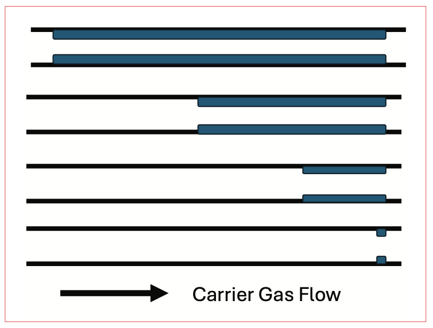
Solvent effect focusing occurs in the column once the solvent band containing dissolved analytes is deposited at the column head and spread out. It is essentially the reverse of band broadening in space. As seen in Figure 4, the solvent band containing analytes is spread over a significant length at the column head. As the carrier gas flows from the inlet, the volatile solvent evaporates, but the less volatile analytes do not; they remain dissolved in the solvent. As the solvent evaporates, the solvent band becomes smaller. This process continues; the solvent band becomes smaller, and the analytes are concentrated into a narrow band. Eventually, the solvent has all evaporated, leaving behind a narrow plug of sorbed analytes in the stationary phase. Solvent effect focusing is most useful for analytes that are relatively close in volatility to the solvent and less subject to thermal focusing. For solvent effect focusing to be effective, the initial column oven temperature must be below the normal boiling point of the solvent to ensure that the solvent vapor, as it exits the inlet, is condensed on the stationary phase at the column head; if the solvent vapor is not condensed, there is no solvent effect focusing. This is the main reason why nearly all methods employing splitless injection also use temperature programming.

FIGURE 4: Steps in solvent effect focusing.

Splitless injection is a complex process. In Part I of this series, we saw the reasons, especially for trace quantitative analysis, that splitless injection is so useful and popular. In Part II, we see that splitless injection is a complex process, involving multiple band broadening and focusing mechanisms, each of which can either contribute to separation or harm it. We must consider band broadening in time, as splitless injection can require up to 1 min to complete, and band broadening in space, as the injected solvent band condenses in the column over a wide space. We then must consider focusing methods: thermal focusing and solvent effect focusing, which are the main reasons why splitless injection and temperature programming are almost always used together. Careful consideration of band broadening and focusing mechanisms provides the fundamental ideas that lead to splitless method optimization, which will be addressed in Part III of this series.

References

(1) Snow, N. H. Optimizing Splitless Injections in Gas Chromatography Part 1: What It Is and What Happens When We Inject? LCGC International 2024, 1 (8) 18–21.

(2) Grob, K. Split and Splitless Injection for Quantitative Gas Chromatography: Concepts, Process, Practical Guidelines, Sources of Error; John Wiley and Sons, 2007.

(3) Solvent Expansion Calculator, Restek website. http://www.restek.com/solvent-expansion-calculator (accessed 2025-01-16).

(4) GC Calculators and Method Translator Software, Agilent website. http://agilent.com/en/support/gas-chromatography/gccalculators (accessed 2025-01-16).

About the Author

Nicholas H. Snow is the Thomas and Sylvia Tencza Professor and Chair in the Department of Chemistry and Biochemistry at Seton Hall University, and an Adjunct Professor of Medical Science. During his 30 years as a chromatographer, he has published more than 70 refereed articles and book chapters and has given more than 200 presentations and short courses. He is interested in the fundamentals and applications of separation science, especially gas chromatography, sampling, and sample preparation for chemical analysis. His research group is very active, with ongoing projects using GC, GC–MS, two-dimensional GC, and extraction methods including headspace, liquid–liquid extraction, and solid-phase microextraction.

Nicholas.Snow@shu.edu