On Replication in Biopharmaceutical Analysis

The landscape of biopharmaceutical analysis features different analytical requirements in terms of instrumentation and type of analysis (QC, RTRT, and in-process). One of the questions that often crops up for routine analysis is “How much replication is enough?” Should all the samples be run in triplicate irrespective of the type of analysis, or does the type of analysis (such as charge or size variants) have any bearing on the number of optimal replicates?

There are various factors that the user needs to consider in the matter of biopharmaceutical analysis—first, the objective of replication, and second, the trade-off with respect to cost and time. Ideally, the number of replicates should be large enough to adequately represent the variability present, but not so large that the information gained is unjustifiably expensive with respect to the costs (such as instrument time, analyst time, consumables, and samples). The optimal replication applicable to each type of analysis would therefore lie somewhere in between. For any given sample, one must also consider the sources of variability at play. Although some of these sources would be generally applicable to all types of analytical assessments (including analyst-dependent and system-dependent variabilities), some may be unique to the dynamics of a specific biomolecule, such as changes occurring during analysis (stability related). Traditional data accumulated for a specific analysis and molecule over time can help understand and evaluate effective replication numbers.

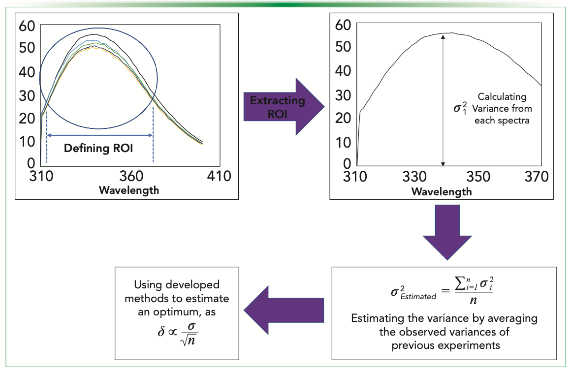
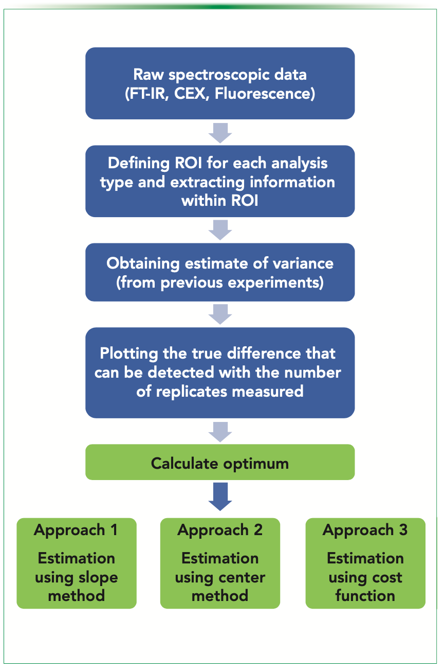
In this article, we use data generated in our laboratory for a published biosimilarity exercise on marketed trastuzumab biosimilars in order to understand and illustrate how the optimum replication number might be influenced by a) the analysis type; and b) devised strategies for efficient utilization of resources to estimate replication number for a given analysis type (Figure 1) (1).

FIGURE 1: Strategy for the estimation of the optimum replication number.

Errors

Blocking and randomization are used in statistical experimental design to balance variability and measure size. After calibrating the equipment and validating the method to reduce variation due to nuisance variables, replication is required to increase the experiment’s informative power. The size of the experiment can be influenced by increasing or decreasing the number of replicates (2).

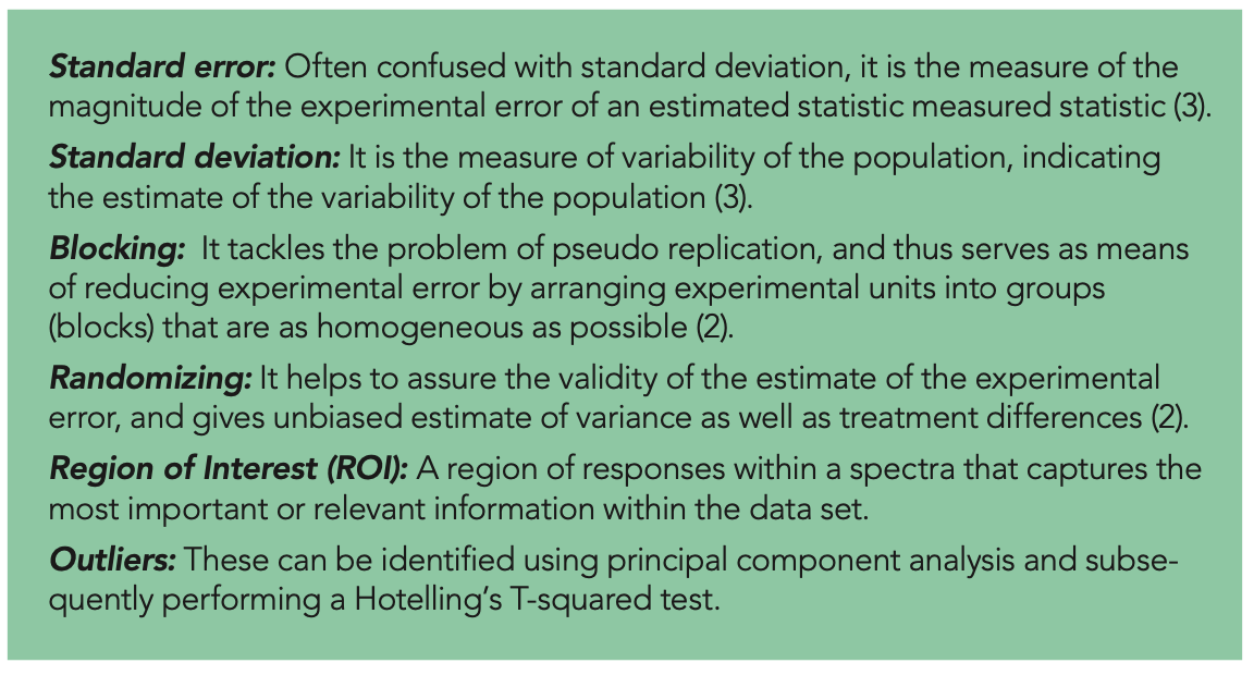
Increased replication helps to reduce the standard error, which is a measure of the magnitude of the experimental error of an estimated statistic. In contrast to the standard deviation, which relates to the inherent variety of observations within individual experimental units, the standard error refers to random fluctuations of a total estimate. By increasing replication, the standard error can be made arbitrarily small. This implies we want a standard error that is small enough to draw reasonable inferences, but not too small.

Types of Error

Type I Error

Type I error is when you declare an effect to be real, and, in reality, it is zero. Setting this to a certain value is usually represented by selecting a value for α (alpha), where α limits this kind of error to a related percentage of probability. Therefore, type I error is also sometimes called alpha (α) error. Similarly, type II error, which will be discussed in the following section, is regarded as beta (β) error (4).

It bears mentioning that simply protecting against type I errors may not be sufficient. Samples of sufficient size may nearly ensure statistical significance, regardless of how little the difference is, as long as it is non-zero. Assuming we only want to discover differences that are important in practice, we add an extra precaution against a type I error by avoiding employing sample sizes greater than those required to defend against the second kind of error—the so-called type II error.

Type II Error

Type II errors occur when an effect is genuine, but is neglected. When the replicates vary slightly, such a failure may not be significant. Only when the disparity is significant does it become problematic. The second step is specifying the probability of actually detecting it. This probability (1-β) is called the power of the test. The quantity β is the probability of failing to detect the specified difference to be statistically significant, and therefore this error is also sometimes called a beta (β) error.

Calculating the Size

Mathematically, the size of the experiment depends on the estimate of variance (σ²); the true difference (δ) that we are set out to detect; the effect of assurance with which it is desired to detect the difference (the power of the test); the significance level that will be utilized in the experiment; and the type of test being necessary (as in whether a one-tail or two-tail test). The required sample size, n, is given by the following formula:

By rearranging equation 1, we can get the true difference, δ, in terms of size n, for an estimated certain variance as:

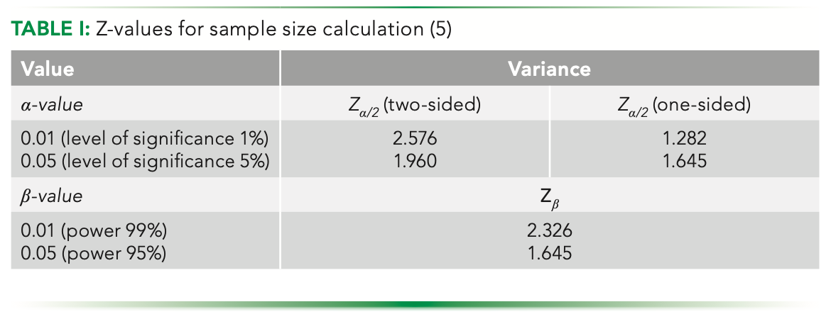
where Z_α/2 and Z_β are the type I and type II errors, respectively, the values for which can be found in the Z tables from most standard books on statistics (see Table I).

In the following, we illustrate this approach using examples from three routine analytical techniques used in biopharmaceutical analysis—namely, Fourier transform infrared spectroscopy (FT-IR), cation exchange (CEX) chromatography, and fluorescence spectroscopy (FLR). For each of these methods, the considered readings were taken in respective region of interests (ROIs) while estimating the variance, and the final estimate was made by averaging the obtained variances for replicates in each batch for all the originator and biosimilars being considered here in this study. For FT-IR, the original data measured over 400–4000 cm^-1 was taken in the ROI of 1400–1900 cm^-1. In CEX, the readings were over 0–20 min; the considered ROI is 9–17 min. In the fluorescence data, the ROI was taken in just the Gaussian curve, and it was between 310–370 nanometers. After estimating the averaged variances, we can find the relation of how the δ changes with the replicate number. Here, we study two confidence intervals of 95% and 99% for each of the errors.

With the Z values and estimate of the variances, we can obtain a curve for δ versus the replication number (Figure 2). Starting with FT-IR data (Figure 2a), we obtained an average variance of 7.052e^-06 in the observed ROI. This helps us visualize the increase in the impact of higher replication on the ability of capture differences between the given data sets. Similarly, the observed variances (averaged) in CEX (Figure 2b) and fluorescence (Figure 2c) data were 117.088 and 77.153, respectively, for the considered ROIs in each. As the relationship between the two axes is the same (inverse root of replication), the order of values on the vertical axes corresponds to the order of response measured for the experiments, from which the variances were calculated and averaged. The effect of increasing the power of errors (moving from 95% confidence to 99% confidence) reflects an upwards shift of the curve along the y-axis, implying that the overall trend of the curve remains the same, and that the true difference that could be captured is more at each particular replication number.

FIGURE 2: Curve showing increase in the impact of higher replication on captured differences. Ordinate data scales are different for (a) FT-IR, (b) CEX, and (c) FLR.

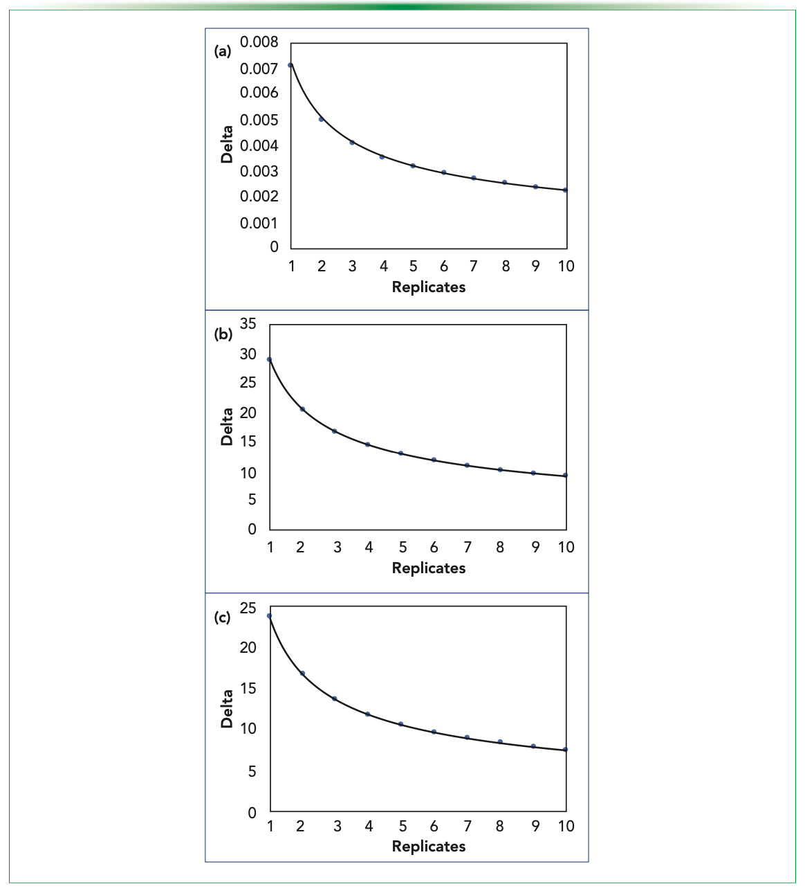
The relationship between delta and replication is non-linear and exponential in nature, meaning that, beyond a certain number of replicates (thereafter referred to as optimum replication R_o), the cost associated with replication is greater than that of the value of the information gained. It would then help to have a mechanism to decipher the value of R_o for a given analyses. To achieve this, we need methods that inherently consider the estimated variance and the power of tests used.

Estimating an Optimum (R_o)

While estimating an optimum, it is important that the devised methods capture the effect of the estimated variance for the different data sets, and yield a number accordingly. For example, R_o may differ among the different chromatographic and spectroscopic techniques. Keeping this in mind, we explored three approaches to yield an estimate for R_o. The methods essentially exploit the shape of the curve obtained as a function of the relationship between delta and replication number, and are based on exploration of geometrical features (such as slope, center, and deviation from linear relation). We have applied this to three types of data sets commonly obtained in biopharmaceutical analysis—ion exchange chromatography, FT-IR spectroscopy, and fluorescence spectroscopy.

Estimation Using Slope Approach

Physically, the replicate number will be integral, and equation 1 should yield discrete values as the number goes from 1 to 10 (10 has been defined as a maximum here based on general laboratory practices). However, to leverage the curve mathematically, we have considered it to be continuous for this and the subsequent estimation below.

In the slope method, we first look at the overall decrease in the variance over the maximum replication that we could go to (defined here as 10). In graphic depiction, this number corresponds to the line AB in Figure 3a. The plots considered here are for the fluorescence data at 5% significance and 95% power for type I and II errors, respectively.

FIGURE 3: Estimating R_o using the slope method; (a) highlighted values at integral points; (b) absolute difference of slope of the curve w.r.t. the slope of line AB; and (c) red dot indicating the estimated point to be rounded to nearest integer.

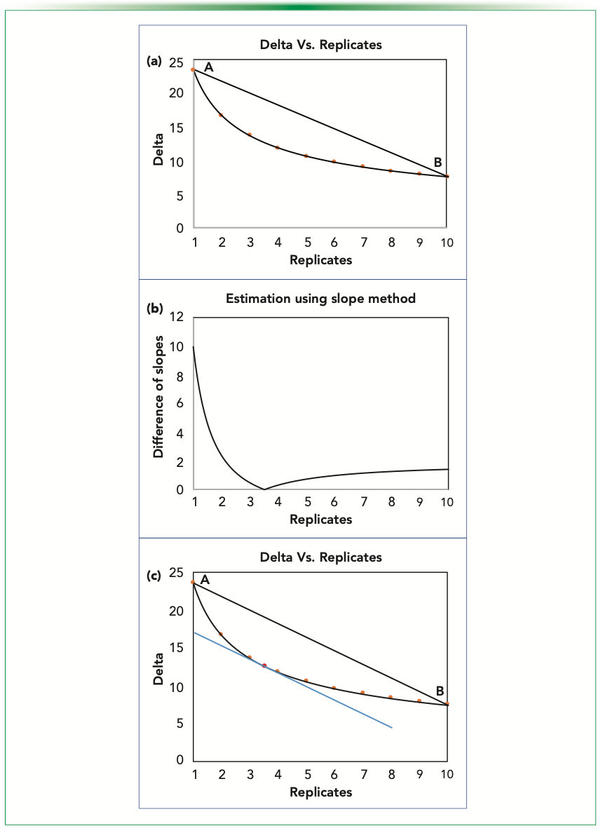
With that line, we find the point on the replicate axis that has a slope equal to that of line AB; one can easily argue that there would indeed exist such a point. Using equation 2, upon differentiating, we get a mathematical expression for the slope in continuous domain as:

Using equation 3, we compare the slopes at each point, and get a number having the same overall decrease of detectable delta over replicate. We plot the difference between the slopes to visualize the trend, and then the minima of it. As depicted in Figure 3b, the minima is found to be at 3.514. Graphically, we will have a tangent with an equal slope as that of AB, as shown in the Figure 3c.

Because we are working in the continuous domain, we will get a positive real number as the estimate that needs to be rounded off to the closest integer for physical consideration. Having done that, we have estimated a number that we can say to be optimum. Here, the closest integral number to 3.514 will be 4, so that is our predicted optimum.

This method of slopes is based upon finding the maximum deviation of the delta values, if the relation was to be linear between them and the replicates with a slope the same as that of a line joining the end points of our considered replication range. It can also be said to be looking at the maximum dip present graphically, as depicted in Figure 4a. The deviation distances should naturally go to a maximum value as it is zero at both ends of the curve.

FIGURE 4: Estimating R_o using the slope method, alternatively seen as deviation distance; (a) the observed dips at integral points seen as parallel lines with optimum at P and (b) plot depicting the trend of the dip.

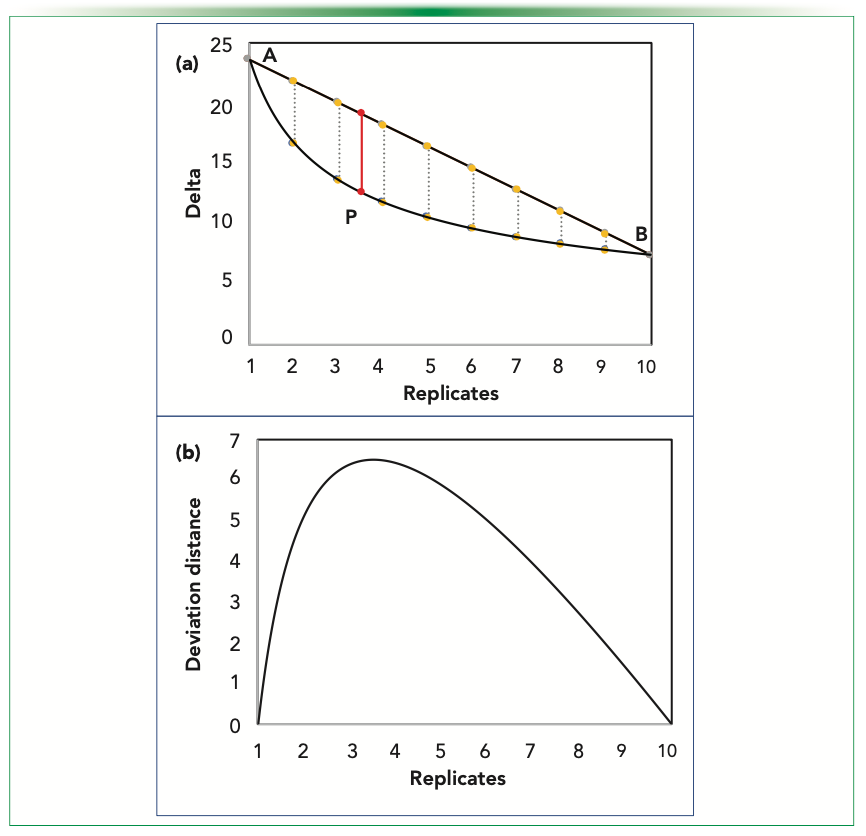
Thus, the continuous deviation values can be plotted, as shown in Figure 4b. Mathematically, it so happens that the numerical optimization function becomes the same upon differentiating while maximizing the deviation distance, resulting in an expression identical to that obtained when the slope was compared. This is basically because of the nature of the function that we are using. The summary of the estimated optimum is as given in Table II.

We see that the predicted optimum number using this method is the same for all spectroscopic methods, thus essentially suggesting that this method has failed to recognize the variance in it, and it predicts a generalized R_o value.

Estimation Using Center Method

Through this approach, we find the center of the curve (the point on the curve that is equidistant from both the ends of the curve). As the point being equidistant from the two extreme ends (as in Figure 5a) are competing with the detectable difference and the replication done, the middle point can be an optimum balancing the two conflicting aspects of the features of the curve.

FIGURE 5: Estimating R_o using center method; (a) estimated point P subtending equal length or angle with the endpoints of line AB; (b) plot depicting the difference of sides from the ends.

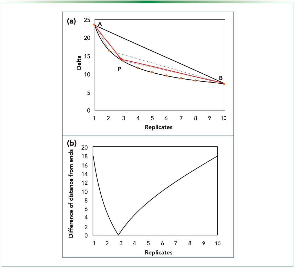
We plot the difference of the distance of the points on the curve and expect a minimum to be there, highlighting the point that is equidistant. Figure 5b shows the variation of the difference of distances for points on the curve from the ends. The minima occur at 2.829. By rounding off, the integral estimate that we get is 3. Graphically, we see that the point of the minima subtends equal angle with the line AB, and will essentially make an isosceles triangle, including itself and the triangle PAB, with PA and PB being the two equal sides (Figure 5a). The summary of the results obtained using this method is shown in Table III.

Therefore, we see that each method yields a unique number based on the variance obtained from the respective technique for a given analysis, providing an appropriate method to make an estimation.

Estimation Using Cost Function

Having seen a couple of methods based on using geometrical aspects of the curve, we now try to develop a cost function that penalizes if the replication number is too high, and incentivizes for the low delta values, so that we anticipate a minimum in the function as we increase replication.

Initially, we proposed a function as equation 4. As n increases, the function value increases. However, at the same time, because of the corresponding decrease of delta values, the function value decreases as well.

Considering this, we can expect a minimum value, but that minima can possibly fall well above our maximum number of replicates taken. This function being explicit in terms of replicate number, upon solving this function mathematically, we get the R_o as equation 5:

We see here that optimum is dependent on the variance that is essentially desired, but the order of variance can be very different for experiments. To handle this uncertainty, we can further modify our function by dividing δ by σmin, where σmin is the lowest variance observed of all the previous experiments; for fluorescence data, the observed minimum in the data set was 48.472. The function then can be written as equation 6:

Mathematically, the optimum for this function can be written to be at:

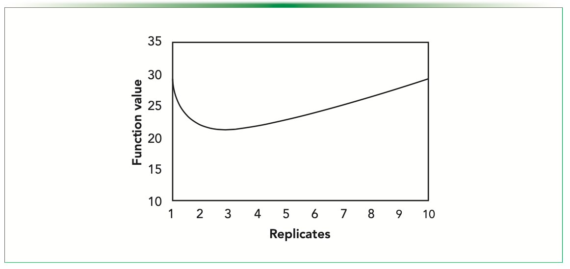
Although we have a mathematical expression, we plot the function and try to depict the minima that must be there. Figure 6 shows the plot of the cost function for fluorescence data (at 5% significance for α, and 95% power for β). We can see that the minimum is in our limit to our maximum range. The summary of the results obtained using this method are presented in Table IV.

FIGURE 6: Estimating R_o using cost function.

Here again, we get a unique number for each experiment, thus being a consistent approach to estimate an optimum with.

Conclusions

Irrespective of the analysis, the general scheme to be followed for R_o estimation is shown in Figure 7, starting from the raw data to the proposed approaches.

FIGURE 7: General scheme for R_o estimation.

R_o estimation approaches can be compared based on effect and the range of relation they share with the estimated variance of a given technique and analysis type, it being the defining feature for the relevance of R_o obtained. While the first approach is insensitive to estimated variance, it could be used as an estimation method where the innate mathematics inherently incorporates the impact of variance (and other such related parameters) over the estimation.

The second approach, while being sensitive to individual technique vari- ance, does not measurably distinguish between confidence for both type I and II errors, as can be seen in Table III.

The last approach based on the developed cost function is both sensitive to technique specific variance as well as the error confidence interval, and thus can be applied across analytical characterization platforms to get a realistic and relevant understanding of the replication required, which is technique and analysis specific based on variances derived from existing analytical data, thus facilitating a more rational approach to defining replication.

Although the work discussed here is in specific context of biopharmaceutical analysis, it would be equally applicable across different domains where chemical data is generated in the form of x and y line plots.

References

(1) S. Joshi and A.S. Rathore, BioDrugs 34, 209–223 (2020).

(2) P. Berthouex and L. Brown, Statistics for Environmental Engineers (CRC Press, Boca Raton, FL, 2nd ed., 2002).

(3) A. Banerjee, U.B. Chitnis, S.L. Jadhav, J.S. Bhawalkar, and S. Chaudhury, Ind. Psychiatry J. 18(2), 127–131 (2009).

(4) D.G. Altman and J.M. Bland, BMJ [Br. Med. J.], 331(7521), 903 (2005).

(5) J. Charan, R. Kaur, P. Bhardwaj, K. Singh, S.R. Ambwani, and S. Misra, Ann. Natl. Acad. Med. Sci. (India) 57, 74–80 (2021).

ABOUT THE CO-AUTHORS

Anurag S. Rathore is with the DBT Center of Excellence for Biopharmaceutical Technology at the Indian Institute of Technology, in Delhi, India. Direct correspondence to: asrathore@biotechcmz.com

Srishti Joshi serves as the Coordinator of Analytical Characterization Division at the DBT Centre of Excellence for Biopharmaceutical Technology at the Indian Institute of Technology under the guidance of Professor Anurag S. Rathore, Department of Chemical Engineering, Indian Institute of Technology, Delhi.

Akshdeep Ahluwalia is a senior undergraduate pursuing a Bachelor's plus Master's, Dual Degree program in Chemical Engineering at the Indian Institute of Technology in Delhi, India.

Jared Auclair is an Associate Dean of Professional Programs and Graduate Affairs at the College of Science at Northeastern University, in Boston, Massachusetts. He is also the Director of Biotechnology and Informatics, as well as the Director of the Biopharmaceutical Analysis Training Laboratory.