Tools for Investigating the Expanding Per- and Polyfluoroalkyl Substances (PFAS) Universe
Per- and polyfluoralkyl substances (PFAS) continue to need novel analytical tools for their proper characterization. Regulatory bodies are lowering the acceptable concentrations for contaminated matrices, requiring state-of-the-art instrumentation to detect sub-ng/L levels. Suspect screening (for known PFAS without certified analytical standards) is becoming more popular as the list of known PFAS grows to thousands of compounds. The methods that currently exist for suspect screening require updating to move them from boutique, study-by-study methods to those that can be adopted more universally to generate transferable data sets. Some of those updates are presented here with the hope that they are adopted by laboratories in industry, government, and academia.
Per- and polyfluoroalkyl substances (PFAS) are a class of compounds characterized by the presence of highly inert carbon–fluorine bonds that impart both oleophobic and hydrophobic properties. These properties have made PFAS useful ingredients in a variety of manufacturing processes, including food packaging, papers and textiles, industrial nonstick coatings, and aqueous film-forming foams (AFFFs) for extinguishing hydrocarbon-based fuel fires. These compounds are sometimes called “forever chemicals,” because they do not break down readily in the environment and those that do (precursors) degrade to more stable end products. The U.S. Environmental Protection Agency (EPA) published a strategic roadmap in 2021 outlining plans to deal with PFAS contamination (1).
The world of PFAS is an exciting avenue of exploration for analytical chemists, because advanced studies involving fate and transport in the environment, ecotoxicity, and treatment can be performed. However, fundamental questions about the detection, quantification, and communication of PFAS results still need to be answered. These challenges bring together separations science, mass spectrometry (MS), data science, environmental engineering, and even public policy.
What constitutes a PFAS molecule has been an ongoing debate. Common among definitions is the presence of a carbon–fluorine bond. However, many molecules can contain a single carbon–fluorine bond and would not be considered PFAS. The main definitions have been built into the PubChem Classification Browser (2), where analysts can generate lists of PFAS according to each definition. Various lists of PFAS have been curated; as a result, there is a lack of consensus because of the varying definitions across lists. The list we chose to use in our studies is one curated by the National Institute of Standards and Technology (NIST) of the United States (3). All lists contain varying amounts of data for each entry, with each having at least the molecular formula. The NIST list contains the molecular structure in a machine-readable format (international chemical identifier [InChI] in this case), and this structure becomes the identifier for each compound. Acronyms and the International Union of Pure and Applied Chemistry (IUPAC) names have been inconsistent across lists; InChIs are a way to unify communication of the results (4). The conversion of InChI keys to draw molecular structures presents an approachable and time-saving exercise in computer coding for the intrepid chemist.
MS has been the choice detector, coupled with gas chromatography (GC) or liquid chromatography (LC), for volatile or non-volatile PFAS analysis, respectively. Most PFAS receiving regulatory scrutiny have been non-volatile, and LC– MS has been the most often used tool.
Targeted analysis of PFAS is done using triple-quadrupole detectors to monitor ion transitions for quantification. The availability of analytical standards has increased greatly over the past 20 years, from almost no standards to mixes where dozens of PFAS can be included in a targeted run. Not all native standards have an exact-matched isotopically labeled surrogate, so some surrogates are borrowed by natives within a PFAS class. It is best to avoid recruiting surrogates from natives where high concentrations are expected. High concentrations will suppress the surrogate signal, which is fine for the exact-matched native but not for a native borrowing the surrogate. For low concentrations, advances in instrumentation and preconcentration steps have led to sub-ng/L levels of detection (LOD) for certain PFAS. Such low levels make contamination an issue not to be underestimated, even in routine targeted analysis.
After targeted analysis, suspect screening and non-targeted analysis are the next frontier in PFAS identification. Suspect screening requires the use of a high-resolution detector, such as a quadrupole time-of-flight (QTOF), ion mobility (IMS), or an orbital trap MS instrument. Mass-to-charge (m/z) ratios are screened against a list of PFAS to look for similar masses. Then, confidence in the identified compound is increased through isotope ratio differences, the presence of diagnostic fragments, and other data acquired. These confidence levels were initially communicated using the scale developed by Schymanski and others for all non-targeted MS work (5). This scale was the framework for a new scale that our team created to communicate confidence of PFAS identification using features specific to PFAS (6).
The growth in awareness of the true number of PFAS has far outpaced the availability of analytical standards for true quantitative analysis. The demand for PFAS research led to the idea of reporting new or suspected compounds in a semi-quantitative way. Most new or suspected PFAS are either part of an existing homologous series, or have only small changes to headgroups. For new or suspected PFAS, one would borrow the calibration curve from a similar compound that does have an analytical standard, assume an equal molar response by the detector, adjust for molar mass differences, and call this a semi-quantitative concentration. This technique assumes that the ionization efficiencies between the suspect PFAS and the borrowed calibration PFAS are similar. Although this strategy worked initially, a number of problems have been found over time. The discovery of new PFAS compounds has outpaced the ability to match them to existing standards.
As studies have become more complex, involving multiple environmental matrices with vastly different PFAS concentrations, the matching had to be altered for different matrices. Different matching schemes are used across the literature, making comparisons across studies difficult. Finally, different laboratories run slightly different analyte lists, making a universal matching scheme unattainable. To address this, we developed a new method to estimate concentrations that we believe can accommodate the rapid growth in demand for PFAS testing and information.
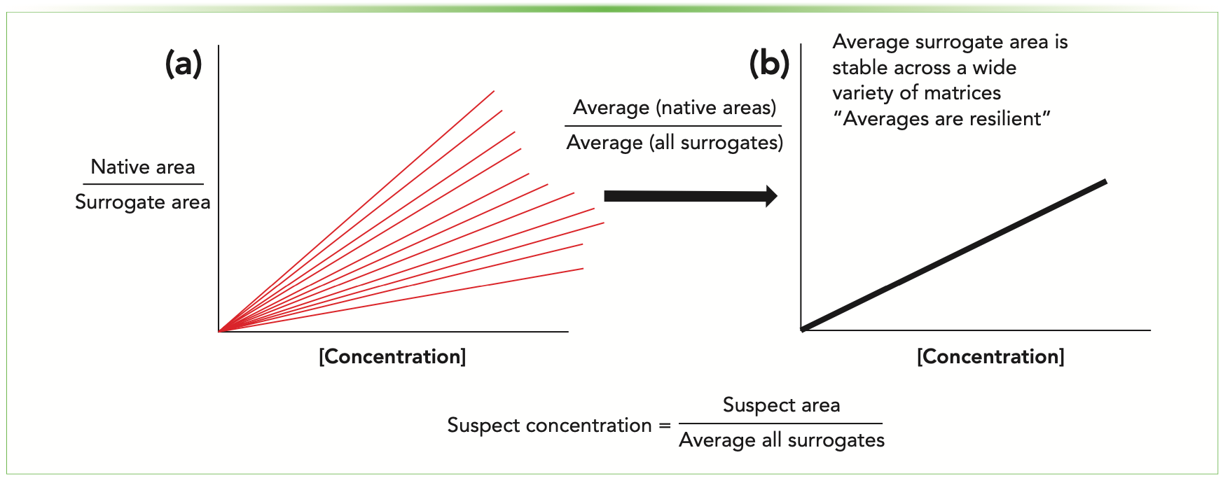
The PFAS curve replaces one-to-one matching with a single, average curve comprising all the PFAS standards run in a particular study (Figure 1). The same curve is used for all suspected PFAS, including non-targeted PFAS where the exact structure and location of functional groups (and thus estimated ionization efficiency) may not be known. This technique was partially inspired by an idea from data censoring, where traditional techniques, such as substitution of values below the limits of quantification (LOQ), presented a false sense of knowledge about the data (7). In the case of one-to-one matching, ionization efficiencies of suspect compounds can only be known using analytical standards, and without those, the ionization efficiencies are an educated guess at best. The single PFAS curve is likely wrong for most suspects, but it is wrong systematically, and if multiple studies use this technique, the estimated concentrations are comparable across data sets. Finally, it is a computationally simple approach compared to one-to-one matching and has a better chance of being adopted by laboratories across government, academia, andindustry. We are currently working on a study using 19F-NMR to measure the total organic fluorine to quantify the variability of this method.
FIGURE 1: Graphic depicting (a) multiple calibration curves and (b) the single PFAS curve for estimating suspect concentrations. One-to-one matching involved estimating which calibration curve would most closely mimic the suspect PFAS. (b) The new technique uses one curve for all suspect PFAS, and would unify semi-quantitative techniques across studies and laboratories.

The details of naming and quantifying PFAS are important when the scale of PFAS contamination is realized. A recent study proposed that most rainwater, even in remote areas, contained PFAS above the health advisory levels set by the U.S. EPA (8). Solutions to this problem will require new thinking and incorporating new methods of data analysis, such as machine learning. The more data can be generated and shared, the better these problems and solutions can be understood. Some of the techniques outlined here should help in streamlining and automating much of that work.
Acknowledgments
The author would like to thank the Strategic Environmental Research and Development Program (SERDP) for funding through grants ER19-1205 and ER20-1375.
References
(1) PFAS Strategic Roadmap: EPA’s Commitments to Action 2021-2024 (U.S. Environmental Protection Agency, Washington, D.C., EPA Report EPA-100-K-21-002, 2021).
(2) National Center for Biotechnology Information, PubChem Classification Browser. https://pubchem.ncbi.nlm.nih.gov/classification/#hid=120 (accessed October 2022).
(3) B.J. Place, Suspect List of Possible Perand Polyfluoroalkyl Substances (PFAS), National Institute of Standards and Technology (2021). https://doi.org/10.18434/mds2-2387
(4) S.R. Heller, A. McNaught, I. Pletnev, S. Stein, and E. Tchekhovskoi, J. Cheminform. 7, 23 (2015). https://doi.org/10.1186/s13321-015-0068-4
(5) E.L Schymanski, J. Jeon, R. Gulde, K. Fenner, M. Ruff, H.P. Singer, and J. Hollender, Environ. Sci. Technol. 48(4), 2097–2098 (2014). https://pubs.acs.org/doi/pdf/10.1021/es5002105
(6) J.A. Charbonnet, C.A. McDonough, F. Xiao, T. Schwichtenberg, D. Cao, S. Kaserzon, et al, Environ. Sci. Technol. Lett. 9(6), 473–481 (2022). https://pubs.acs.org/doi/10.1021/acs.estlett.2c00206
(7) D.R. Helsel, Statistics for Censored Environmental Data Using Minitab and R (John Wiley & Sons, Hoboken, NJ, 2nd ed., 2012).
(8) I.T. Cousins, J.H. Johansson, M.E. Salter, B. Sha, and M. Scheringer, Environ. Sci. Technol. 56(16), 11172–11179 (2022). https://pubs.acs.org/doi/pdf/10.1021/acs.est.2c02765
ABOUT THE AUTHOR
Trever Schwichtenberg is a Postdoctoral Scholar at the Oregon Health and Science University, in Portland, Oregon. Direct correspondence to: trever.schwichtenberg@gmail.com.


Troubleshooting Everywhere! An Assortment of Topics from Pittcon 2025
April 5th 2025In this installment of “LC Troubleshooting,” Dwight Stoll touches on highlights from Pittcon 2025 talks, as well as troubleshooting advice distilled from a lifetime of work in separation science by LCGC Award winner Christopher Pohl.
Study Examines Impact of Zwitterionic Liquid Structures on Volatile Carboxylic Acid Separation in GC
March 28th 2025Iowa State University researchers evaluated imidazolium-based ZILs with sulfonate and triflimide anions to understand the influence of ZILs’ chemical structures on polar analyte separation.


