How Close is Close Enough? Accuracy and Precision: Part II

Modern gas chromatographs are expected to deliver the highest performance levels, but actual performance can suffer due to a number of causes including inappropriate methodology as well as improper instrument setup and poor maintenance. It is always important to keep accurate and complete records of periodic test or validation mixture analyses and any changes to instrument configuration, the methods used, and samples run to help diagnose problems when they occur. Sometimes a problem is obvious, but often something seems to be going wrong while there is no obvious failure. Retention times begin to drift, area counts start to decrease, or repeat results seem more scattered than before. Deciding if these subtle changes are significant is not a trivial task. If there is a significant problem, then additional steps can be taken to diagnose and resolve it. If the problem is insignificant, then considerable time might be saved.

Later on Monday

The first installment of this column series presented a situation in which an initial chromatogram from Monday morning gave retention times that seemed to fall outside the range of expected values based upon observations from the most recent runs obtained on Friday of the previous week. For one peak the average retention time in 10 chromatograms from Friday's data was 14.38 min and the standard deviation of those retention times was 0.011 min. The first run on Monday eluted this peak at 14.41 min; 2.7 standard deviations removed from Friday's average value. At issue was whether this difference between Friday and Monday was significant and required attention, or if this was an acceptable occurrence that could be ignored safely. If the change were significant, a chromatographer might decide that he or she should pay close attention to the instrument in question because its retention times had shifted significantly over the weekend. There are many possible fault conditions that could result in drifting retention times. Is there a septum leak? Is the pressure controller drifting? How stable is the gas chromatograph's oven temperature? Our analyst needs to distinguish a developing or full-blown problem that affects data integrity — in this case our ability to identify peaks on the basis of their retention times — from fluctuations that occur in the course of normal daily operations.

John V. Hinshaw

A conclusion that there is a retention time shift is a weak one, however, for at least two reasons. First, deciding to pursue a potential retention time problem on the basis of a single sample — let alone the first sample on Monday morning — would be a difficult choice to justify. Second, Friday's 10 observations represent a small sampling of a much larger collection of acceptable experimental outcomes for this peak's retention time, which necessarily covers an observation period longer than a single day. Due to normal variations the average and standard deviation of one day's worth of observed retention times could be different than for a more populous set of retention data acquired over the course of a week or a month. Student's t-test, introduced in the first part of this discussion, helps a small data set better model the expected behavior of the larger set that it represents by compensating for the tendency of small sample collections to appear more spread out than the overall population being sampled. In our example, the standard deviation of Friday's 10 samples is assumed to exaggerate somewhat the distribution of the greater population at large. According to this metric, Monday's first retention time was more than 98% likely not to be a member of Friday's data set.

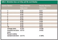
Table I: Retention times on Friday and the next Monday

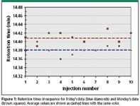
Our technician decides to allow a normal series of 10 consecutive runs to proceed. The retention times of the peak of interest in these runs are given in Table I along with Friday's retention times. Figure 1 shows this data plotted on a run-by-run basis along with the average values for both days, which are plotted as dashed lines. The average values for Monday and Friday are rather close to each other; they differ by only 0.039 min (2.3 s). From this graphical presentation, we can see immediately that the additional nine Monday runs seem to indicate a significant difference between the two days, but how strong a case is this?

Figure 1

Making a Case

To answer the question, "Do the retention data from Friday and Monday differ?" we will turn to statistical analysis of the two data sets and compare them to each other. First, though, we need to rephrase the question so that it reads, "Are the retention data from Friday and Monday both representative samplings from the larger set of all valid retention times for the peak in question?" This introduces the concept of sampling into our discussion. We will assume that there exists a large set of retention time data that includes all the values that are acceptable for simple retention time-based peak identification. If the peak's retention time is a member of this set, then it will be identified correctly. It not, then the peak either will not be identified at all or will be misidentified. Other schemes that help compensate for retention variability are possible, such as relative retention times, but here we will stick to the simplest case. Even though their averages are different, Friday's and Monday's retention times could in fact represent different subsets of members of the same data set. The unpredictability of taking a small number of samples can yield different average values for distinct groups of data which, were we to include many more measurements, eventually would converge.

Nothing is simply true or false in the world of statistics, however, and so we will have to calculate the magnitude of our confidence that the assertion about Monday's and Friday's results is true or false. Then we will be in a position to quantify how well we can expect the chromatographic method to identify the peak. But before we can get to this point, we need to examine the relationship between the experimental data and its range of possible values.

Here we have a challenge that is a core issue in statistical analysis. How do we represent the population of samples at large that we will use for comparisons to our experimental data? We could imagine collecting a large number of retention times over several weeks or months. But by the time we have accumulated experimental data from one or two hundred runs, something inevitably will have changed that makes the newer retention data distinguishable from the older existing values. By definition, these values are no longer members of the larger set of data that we accumulated before a change occurred. If the changes are acceptable — meaning we can adapt to the new retention time by updating the expected time in the method — then we have started a new set of valid retention times to use going forward. Perhaps the column was changed, or just reinstalled in a different instrument. Perhaps a septum leak was discovered and fixed, or maybe a carrier gas pressure controller or the oven temperature was recalibrated. If I condition a column overnight at elevated temperatures, I might expect that subsequent retention times will be reduced slightly due to the removal of retentive contaminants and perhaps, but hopefully not, some of the stationary phase itself. As always, good recordkeeping is critical in such situations. For now, we will continue and assume that there is no such obvious cause-and-effect sequence.

Random Chances

The moving-target characteristic of these real-world situations forces us to rely on assumptions about the nature of the set of acceptable values. At the simplest level, we could assume that our data is in fact completely random. In that case, the order in which the experimental data was acquired should have no effect on the statistics. It would be as if we had a drum filled with a thousand otherwise identical balls numbered with possible retention values. Imagine performing a series of experiments that consist of spinning the drum to randomize the balls, choosing one numbered ball at a time, recording the retention time from the chosen ball, returning it to the drum, and then repeating this operation.

How many balls with each possible retention time shall we put in the drum, so that we can best represent a set of data that models our experience? If the smallest difference is we measure retention times to 0.01 min, then there are 21 possible values ranging from 14.30 to 14.50 min. One scenario places 50 balls with each value in the drum. In this case, there would be an even chance of selecting a ball with any of the possible values. Because we are returning each ball to the drum before choosing another, the chances of selecting a ball with any one value are 1 in 21 or a little over 5%. In other words, this model predicts that it is equally possible for a single retention time measurement to fall anywhere within our chosen range. This behavior clearly does not mimic the retention time data at hand, so what else is going on?

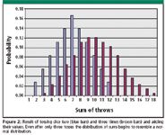
Throwing the dice: Statistics provides a good explanation. Imagine a regular six-sided die. If I toss the die several times, there is an equal chance of 1:6 with each throw that any one of the faces will land on top. This situation is similar to our drum loaded with an equal number of each possible retention time. Now if I add the values of the first two throws of the die to each other (or throw two dice at once and add), the situation changes significantly, although not so much that I will head for Las Vegas. By adding, I have coupled the results of the two throws. At this first stage with two throws, there are six possible ways to obtain a seven: (1, 6); (2, 5); (3, 4); (4, 3); (5, 2); and (6, 1). There are 36 possible outcome pairs from two throws of the die, so the probability of getting a seven is 6/36 or 0.167. There are five chances of getting a five and five chances for an eight, with a probability of 5/36 or 0.134 for either. The number of chances decreases until at the far end there is only single chance of getting a two ("snake-eyes") and a single chance for a twelve, each with the lowest probability of 1/36, or 0.028.

If I throw the die a third time and add the result to the sum of the first two throws, I will have 26 ways to get a nine or a 10, now the most probable outcomes. After three throws, there are 216 distinct possible outcomes, in terms of the order in which a series of three numbers from one through six can be combined, so the probabilities of a nine and of a 10 are both 26/216 = 0.12. The further removed I am from the central values of nine and 10, the lower the probabilities, until I reach a low of 0.0046 for the extreme values of 3 or 18.

Central limit theorem: Figure 2 shows the probabilities of hitting all possible sums for two and three tosses. If you have ever looked into what happens when two dice are tossed in a casino, the triangular distribution for the outcomes of two throws will look familiar. The distribution of the sums for three tosses should look somewhat familiar to chromatographers. If I were to continue tossing the die and add the results of four or more additional throws I would very closely approach a normal distribution curve which also is, and not by coincidence, a good model for chromatographic peaks. Fortunately for my spreadsheet, which at this stage would require 6⁷ = 279,936 cells to hold the results, we will not pursue the topic any further in this direction. 216 possible outcomes are enough to keep track of.

Figure 2

A collection of experimental observations taken in the context of many random linked variables, such as multiple serial tosses of a die, tends to approach a normal distribution in an effect called the central limit theorem. The peak-broadening process in a chromatographic column mimics this type of randomness as solute molecules partition in and out of the stationary phase, performing a truly huge number of "tosses." Other asymmetric processes occur in a column as well, which is why a chromatographic peak only approximates a normal distribution.

For our retention data, if each observed single retention time is the result of a series of random events then, according to the central limit theorem, a collection of retention values should fall into a normal distribution. This is important for understanding the relationship between the Monday and Friday data sets. The collection of the mean values of a number of, in our example, daily data sets will take on a distribution that closely mimics the mean and distribution of the set of all possible retention time values for this peak. However, some of these values might lie outside the range of what is acceptable in the context of identifying the peak by its retention time.

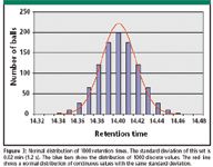
We can use this kind of statistical model in situations where the overall population is unknown but its statistical behavior can be characterized, as long as the processes that determine the variability in the data are random. In the case of our drum, we will choose retention times that approach a normal distribution. Figure 3 shows this distribution for 1000 retention values that cover the range of our peak of interest. The most numerous value is 14.40, with 199 representatives. The next numerous groups lie plus and minus 0.01 min away from the mean, with 176 apiece, followed by plus and minus 0.02 min with 121 representatives each. On a percentage basis we will find 55.2% of the values fall within 0.01 min; 79.4% within 0.02 min; 97.8% within 0.04 min; and 100% within 0.06 min. This distribution is slightly different that the normal distribution (the red line in Figure 3) because we have a set of 21 discrete values in the drum whereas the normal distribution assumes that the sample values are continuous. The flattening effect of discrete sampling on the distribution curve is visible.

Figure 3

Evaluating the Data

We still need to determine how well this distribution of possible retention times represents the set of acceptable values. How do the chromatographic method requirements affect the standard deviation of this data set? What is the minimum confidence level that we can accept for peak identification? Once these statistical parameters are determined we can proceed to evaluate Friday's and Monday's data in a defined context. A future installment of "GC Connections" will continue this discussion.

John V. Hinshaw

"GC Connections" editor John V. Hinshaw is senior staff engineer at Serveron Corp., Hillsboro, Oregon, and a member of LCGC's editorial advisory board. Direct correspondence about this column to "GC Connections," LCGC, Woodbridge Corporate Plaza, 485 Route 1 South, Building F, First Floor, Iselin, NJ 08830, e-mail lcgcedit@lcgcmag.comFor an ongoing discussion of GC issues with John Hinshaw and other chromatographers, visit the Chromatography Forum discussion group at http://www.chromforum.com.

References

(1) J. Hinshaw, LCGC 24(9), 996–1002 (2006).