Count the Cost, Part III: Increasing Resolution by Changing Selectivity

Several variables can be used to change selectivity in a liquid chromatography (LC) separation. Here we compare the variables in an effort to prioritize which experiments will be most effective.

This is the third in a series of “LC Troubleshooting” installments that consider how we can use the fundamental properties of chromatographic separations to estimate the impact of different variables on liquid chromatography (LC) separations. In the first installment (1) we looked at the column plate number, N, and saw that it was not as useful a tool as we might guess, but concluded that a column with a plate number of N ≈ 10,000 is a good place to start. Last month (2), we considered retention, expressed as the retention factor, k. It is best to adjust retention for 2 ≤ k ≤ 10. If the sample won’t fit in 1 ≤ k ≤ 20, a gradient method is likely a better choice.

As in the previous two installments, we’ll use the fundamental resolution equation as a guide:

This month we’ll focus on selectivity, α, (or peak spacing) as expressed in term ii of equation 1, where α is the selectivity factor between two peaks with k-values of k₁ and k₂:

Several variables can be adjusted to change α. It is not surprising that some of these variables are more effective and some are easier to change than others. By looking at the effects of different variables on the separation, we can “count the cost” of different choices and choose a balance of the various costs (effectiveness, time invested, expense, and so forth) that fit our requirements.

Orthogonal Separations

When we focus on selectivity during LC method development, we are looking for ways to move peaks relative to each other. This means changing values of α (equation 2) by changing the k-value of one or both peaks under consideration. When more than two peaks are present, it may be necessary to move several peaks relative to each other so that satisfactory separation is obtained. As part of the process of improving selectivity, we’d like to choose a variable (for example, solvent type or pH) that has a high probability of making the desired change. One way to compare changes in selectivity is to plot the retention of the various sample components, expressed as log k, for two different variables, as in Figure 1.

Figure 1: Comparing retention between two conditions. (a) Two variables with similar (“equivalent”) retention; (b) two variables with quite different (“orthogonal”) retention. See text for details.

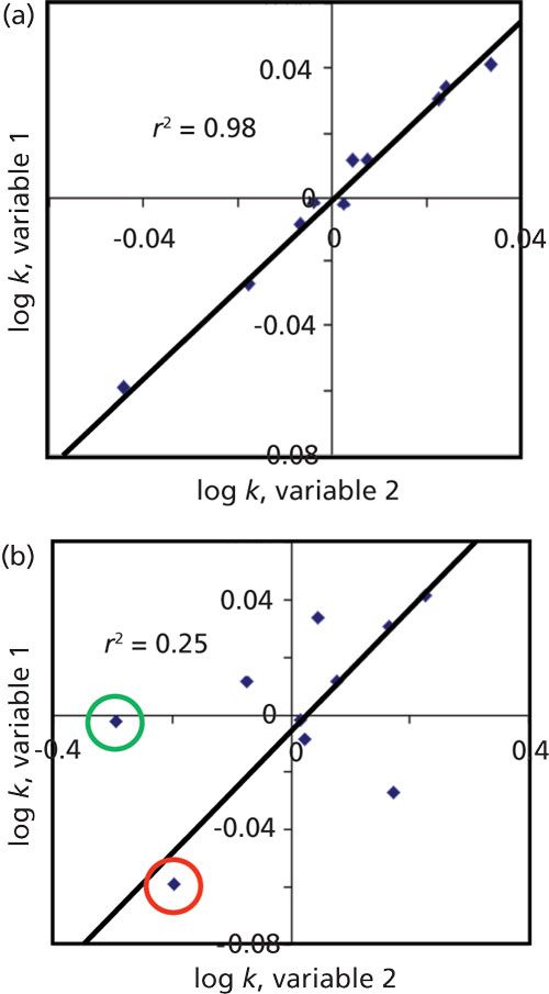
In Figure 1a, the retention of the sample components (blue diamonds) falls close to a straight line, with a coefficient of determination, r², of 0.98. If the slope of the line were 1.0, all components would have the same retention with either variable 1 or variable 2. If r² is close to 1, but the slope is not, the relative retention would be approximately the same, but little or no change in α would be observed. When the coefficient of determination is close to one, we can refer to the separation conditions as equivalent. We might see this if the retention on two different C18 columns were compared. This approach would be desirable if we want two columns that can be used interchangeably, with one of them designated as a backup column for a method. However, this is not a desirable situation if we want to choose a variable that will improve the separation of a hard-to-separate peak pair.

Figure 1b shows more scatter for the points around the trend line than Figure 1. This might occur if we changed the organic solvent (B-solvent) type in a reversed-phase method, where variable 1 is acetonitrile and variable 2 is methanol. Note that when two adjacent points lie on opposite sides of the trend line, a retention reversal has occurred for those two peaks. For example, the point circled in red is eluted before the one circled in green with variable 1, whereas it comes out second with variable 2. As the scatter about the trend line increases r₂ drops, the likelihood of significant changes in relative retention (selectivity) increases, also. When the separations under two conditions are quite different, we refer to the separation as orthogonal. (Yes, technically to be orthogonal, the coefficient of determination should be zero, but this is extremely unlikely with two chromatographic conditions.)

Orthogonal Leverage

Although we could use r², we get a better measure of the scatter of the points, as in Figure 1b, as a function of the standard error of the curve, which for the present discussion I’ll call “orthogonal leverage.” Orthogonal leverage is the power of a variable to make significant selectivity changes for reversed-phase separations. 

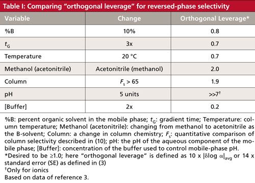
In Table I, I’ve summarized orthogonal leverage data for the common variables we use to control reversed-phase separations. This table is based on a large database of chemically diverse compounds under different chromatographic conditions (see reference 3 for more discussion). When the orthogonal leverage for a specified change in a variable is ≥1, it is a good choice to try to change α for hard-to-separate peaks. Yes, this is an average number that may or may not apply to a specific sample, but in our “count the cost” series, we’re seeking knowledge that will allow us to choose conditions that increase the probability of success as well as learn which conditions are likely to be a waste of time. In each case, data are shown for an arbitrary, but experimentally reasonable, change in the variable (3). Let me next briefly interpret the data of Table I.

%B and t_g

%B refers to the percentage of organic solvent in a reversed-phase mobile phase, most commonly methanol or acetonitrile. In the discussion of k (2), the Rule of Three was mentioned: We can expect approximately a threefold change in k for a 10% change in the B-solvent. This percentage is a reasonable amount of change without being excessive. We can see that this gives an orthogonal leverage value of 0.8, which is less than our target value of ≥1. However, 80% of the way to our goal isn’t bad, and as we know from experience and the discussion of k last month (2), many times a change in %B is sufficient to pull two peaks apart. Also, this change is very easy, so even though it is not as effective as some other variables, it usually is worth pursuing. A threefold change in the gradient time, t_G, will have a similar effect on a gradient method as a change of 10% B does in an isocratic one (4–7). The two changes also have approximately the same effect on orthogonal leverage (0.7 versus 0.8). A change in gradient time is easy and reasonably powerful, so again we choose easy over powerful and often implement a change in gradient time early in the method development process.

Column Temperature 

A change in the column temperature can change the selectivity of a separation (8) because of the affect of temperature on k and mobile-phase pH. A change in temperature of 20 °C gives us an orthogonal leverage of 0.7. Once again, this value is less than the desired ≥1, but because it is easy, similar to a change in %B or t_G, it often is a variable we try early in the method development process.

Another reason that we often choose to investigate %B or t_G and °C early in our investigations is that they are easily modeled based on two experimental values, much like we saw for k in (2). Thus experimental runs at two values of %B, t_G, or °C allow prediction of k and α for other values of that variable. Counting the cost of the experiments, these are very high value, low cost choices.

Methanol–Acetonitrile 

We all know from experience, as well as other “LC Troubleshooting” installments (for example, reference 9), that a change from using methanol to acetonitrile (or vice versa) as the mobile-phase organic component usually has a significant change in the peak spacing of the chromatogram. This effect is reflected in the value for orthogonal leverage in Table I of 2.0, twice the minimum desired target of ≥1. However, although the solvent swap is powerful, it can create such large selectivity changes that we may have trouble figuring out which peaks correspond between the methanol and acetonitrile chromatograms. We have to balance this challenge against the power of moving the peaks. As a result, we often delay investigation of the effect of solvent type changes until we have checked out the easier, but less-effective variables noted above.

Column 

A change from one column to another can have a wide range of results, varying from little or no change in the separation to large changes in α. The label on the column does not necessarily give us enough information to make the decision. However, there are now online databases, such as the one discussed in reference 10, that can quantify the differences between columns, making the choices much easier. Table I shows that the right choice of columns (F_s > 65 according to reference 10) can have a very strong influence on the orthogonal leverage (1.9), approximately the same as changing the solvent type (2.0). As with solvent type changes, however, the change in the chromatogram may be too large when the column is changed. Another drawback of column changes is that they are expensive and discrete. That is, two columns may be compared, but it is not possible to interpolate between two columns, as it is with solvent blends, %B, t_G, or °C. For these reasons, column changes often are delayed until other variables have been tried.

pH 

Changes in the mobile-phase pH can have dramatic effects in changes in selectivity, as reflected in the orthogonal leverage of 7 or more for a five-unit change in pH. However, pH changes work only for ionizable compounds, so this variable is not universal and may have only marginal results on a sample of unknown compounds if some or all are neutral. As was seen in a recent “LC Troubleshooting” installment (11), care has to be taken with pH adjustment to pick an appropriate buffer for the desired pH.

Buffer Concentration 

Buffer concentration in the mobile phase is one of the variables when pH is used to control selectivity. Other than generating a minimum buffering strength (typically 5–10 mM), changes in buffer concentration have little effect on the separation, as reflected in the orthogonal leverage value of 0.2. This one’s easy in the count the cost choices-don’t bother. However, if you are working on an ion-exchange or hydrophilic-interaction chromatography (HILIC) separation, buffer concentration can be a very important variable, so don’t dismiss it as useless for all LC methods.

Other Influences

Table I summarizes the orthogonal leverage for several common variables. This is good information, but it does not tell the whole story, because there are other factors involved in prioritizing which variable to choose first in the method development process. One way of looking at this is expressed in Table II.

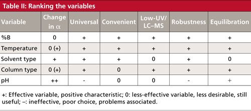
In Table II, I’ve chosen the five important variables for isocratic separations from Table I and added a few more bits of data. I have somewhat arbitrarily assigned a value of + (a good choice, powerful in changing selectivity), 0 (OK, but not great), or - (weak or ineffective, or has major problems). Let’s look quickly at some highlights.

%B

If we consider acetonitrile as the B-solvent, we see that it is OK, but not great, in changing α (reflected in the orthogonal leverage of 0.8 in Table I), but changes will work for all compound types (universal), it is easy, works well down to 200 nm and is compatible with mass spectrometry (MS) detectors (for use in LC–MS), is easily reset (robust), and equilibrates quickly (an advantage for gradients and for screening experiments). So, although it isn’t the most powerful variable, it has good marks in most categories and is easy to change, usually making it my first choice when exploring selectivity.

Temperature

It is easy to think of column temperature as a variable of marginal power (orthogonal leverage of 0.7), mainly affecting retention. However, if ionizable compounds are present, it can mimic changes in pH and can be a powerful variable in adjusting selectivity. This happens often enough that I put it near the top of the variables I investigate. You can see all the other properties of temperature are good.

Solvent Type

A change in solvent type shows pluses in most categories. Care does need to be taken for work at low wavelengths in an ultraviolet (UV) detector. Acetonitrile is good down to 200 nm, but for gradients below 220 nm, methanol may have excessive baseline drift. Changing from one solvent to another (equilibration) may take a bit longer than other changes, but it is not a show stopper.

Column Type

Changing from one column type to another can be a powerful way to change selectivity, but it is usually best when guided by a quantitative column selectivity tool (10). Unless you have a valve-switching setup on your LC system, exchanging one column for another is a bit inconvenient, but other than the cost of buying another column, this variable has few drawbacks.

pH

As discussed in the previous section, pH can be the most powerful way to change a separation, but only works for ionizable compounds. It takes more effort to make up a new buffer than to change temperature or solvent. We have to ensure that the buffer is compatible with the detector: Phosphate works well down to 200 nm with a UV detector, but will cause a snowstorm in a LC–MS system. Unfortunately, improper selection of the buffer or pH can make method robustness a problem.

Two Strategies

We can use the information discussed above to approach selectivity adjustment in method development in two different ways. If we want to do some quick screening experiments to determine if the different variables will be effective for our particular samples, we could pick variables that have large values of orthogonal leverage in Table I. For example, we could screen two columns with two solvents at low and high pH (2³ = 8 experiments total) to choose initial starting points. On the other hand, if we want to fine-tune selectivity, it usually will be easier to start with %B (or t_G for gradient methods) and temperature, because they are easier to fine-tune and the results of two experiments for a variable allow us to predict retention under other conditions.

Summary

We might summarize the discussion of counting the cost in LC method development with the familiar statement, “work smarter, not harder.” Equation 1 helps us evaluate the impact of N, k, and α on the separation. A column with N ≈ 10,000 usually is a good place to start; changes in column length and particle size are easily calculated without additional experiments. Next, adjust retention for 2 ≤ k ≤ 10 or 1 ≤ k ≤ 20 to get “good” chromatography. Fine-tuning k to adjust α by changes in %B or temperature often will give the desired separation. When choosing which variable to explore for further changes in α, we have to balance the cost (both time and money) against the effectiveness (orthogonal leverage) and the ease of making the adjustment; Tables I and II can help guide these decisions.

Today’s business demands often do not give us the luxury of taking as much time as we would like when developing a LC method. It is more important than ever to pause before starting a method development project and count the cost of a proposed strategy. We need to take as little time as possible to develop fast, robust, and accurate methods. There are many ways to do this wrong, but with advanced planning we can make good choices that will minimize wasted time.

References

1. J.W. Dolan, LCGC North Am. 35(3), 170–173 (2017).
2. J.W. Dolan, LCGC North Am. 35(4), 240–245 (2017).
3. J. Pellett, P. Lukulay, Y. Mao, W. Bowen, R. Reed, M. Ma, R.C. Munger, J.W. Dolan, L. Wrisley, K. Medwid, N.P. Toltl, C. Chan, M. Skibic,K. Biswas, K.A. Wells, and L.R. Snyder, J. Chromatogr. A1101, 122–135 (2006).
4. J.W. Dolan, LCGC North Am. 31(3), 204–209 (2013).
5. J.W. Dolan, LCGC North Am. 31(4), 300–305 (2013).
6. J.W. Dolan, LCGC North Am. 31(5), 382–389 (2013)
7. J.W. Dolan, LCGC North Am. 31(6), 456–463 (2013).
8. J.W. Dolan, LCGC North Am. 20(6), 524–530 (2002).
9. J.W. Dolan, LCGC North Am. 28(12), 1022–1027 (2010).
10. J.W. Dolan, LCGC North Am. 29(3), 236–244 (2011).
11. J.W. Dolan, LCGC North Am.35(1), 22–28 (2017).

John W. Dolan

“LC Troubleshooting” Editor John Dolan has been writing “LC Troubleshooting” for LCGC for more than 30 years. One of the industry’s most respected professionals, John is currently a principal instructor for LC Resources in McMinnville, Oregon. He is also a member of LCGC’s editorial advisory board. Direct correspondence about this column via e-mail to LCGCedit@ubm.com