Classifying Chromatographic Systems by Clustering

The aim of clustering is to classify objects so that similar objects are grouped together and dissimilar objects are found in different groups, called clusters. The starting point is always a data table in which objects (samples, substances, chromatographic systems...) are described by several characteristics.¹ One example is when samples are described by areas under the peak or concentrations of several substances. If the analyst finds that certain clusters of samples can be distinguished from others he will assign them to different origins, for example. In other instances, such groups are not expected but classifying the samples according to their similarity helps to better understand the data. In effect, splitting the samples into groups of similar ones facilitates the interpretation by observing what the pattern of variables is for sets of closely related samples and what differentiates them. This is, in fact, the way the human brain functions intuitively when confronted with complex data.

Another application consists of classifying substances according to their retention behaviour. The characteristic describing the substances is then a retention parameter in several chromatographic systems. The inverse is also possible: chromatographic systems are classified according to the retention behaviour of representative substances. This is the example we will develop further in this column.

Classifying Chromatographic Systems

Many stationary phases and still many more combinations of stationary and mobile phases are available. Selecting those that would be good starting points for the development of a specific method is far from evident. It would help to have a restricted set of chromatographic systems (CS) that together serve as potential starting points in method development. The restricted set should consist of systems that are complementary and possess the most diverse selectivity characteristics possible. In chemometric terminology, the CS should be maximally orthogonal (i.e., have the most diverse selectivity), meaning the retention of a set of representative substances is uncorrelated. Such CS are called orthogonal systems further. The term orthogonal is a mathematical term, which means not correlated: the retention parameters of a set of substances chromatographed in two such CS are not (or rather, as little as possible) correlated. One approach is to classify the CS so that CS with similar characteristics (i.e., CS with highly correlated retention characteristics) are found in the same class. Then one or a limited number of systems from each class are selected. The resulting selection would then consist of a set of dissimilar or orthogonal CS.

A Numerical Example

Van Gyseghem et al. determined retention factors for 68 pharmaceutical substances in 11 chromatographic systems (CS) and applied clustering to those data.² The CS are gradient elution systems. To give an idea of the systems used, CS10 is a Suplex pKb-100 column with a gradient of acetonitrile/0.04 M sodium phosphate buffer pH 3.0 from 10:90 to 70:30 (v/v) % in 8 minutes at a flow-rate of 1 mL/min. To explain step-by-step how to perform the clustering, we will apply it to 5 of the 11 CS extracted from that reference. They are called CS3, CS6, CS7, CS9 and CS10. With appropriate software, it is possible to handle much larger data tables: it is no problem to classify a few hundred objects.

(Dis)similarity Measures

To classify the CS in groups, it is necessary to measure the similarity between them. Many (dis)similaritymeasures have been described, the main ones being the Euclidean distance and the correlation coefficient. In the present instance the similarity is based on correlation, since the eventual aim is to select maximally orthogonal (i.e., minimally correlated) systems. However, in most other clustering applications, the Euclidean distance is preferred. The differences between the two will be discussed in the next practical data handling column.

The (Dis)similarity Matrix

The (dis)similarity between all pairs of CS is computed. Instead of working with the correlations as such, we will, to avoid negative numbers, work with 1 - |r| as the dissimilarity value and delete the decimal point to obtain a simpler presentation. The computations lead to a matrix, here a dissimilarity matrix, with dimensions n × n (n = 5). The matrix is symmetrical because the dissimilarity between object 1 and object 2 is equal to the dissimilarity between 2 and 1. For this reason it is usual to show only half of the matrix. Table 1 is the dissimilarity matrix for our example.

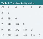
Table 1: The dissimilarity matrix.

Clustering Algorithms

In this first column about clustering we will describe only one of the many clustering algorithms, namely hierarchical agglomerative average linking. The algorithm starts by agglomerating the pair of objects with the smallest dissimilarity (84 between CS6 and CS10). These are now considered to be one object, which we will call 6, 10. In clustering language they are linked together. The dissimilarities between the new object and the remaining objects are the averages of the respective dissimilarities between objects 6 and 10 and each of the remaining objects, which is why the method is said to employ average linking. For instance, the dissimilarity between object 6, 10 and object 3 is equal to (dissimilarity between 6 and 3 + dissimilarity between 10 and 3)/2 = (581 + 673)/2 = 627. The dissimilarities between the remaining objects, other than 6 and 10, remain unchanged. The result is a reduced dissimilarity matrix with dimensions (n - 1) × (n - 1) (Table 2).

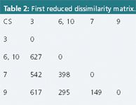
Table 2: First reduced dissimilarity matrix.

This new matrix is further sequentially reduced in the same way. The smallest dissimilarity is found to be 149, leading to the creation of a new object 7, 9, the averaging of dissimilarities involving CS7 and CS9 and the reduction of the matrix with one column and one row. The new matrix is shown in Table 3(a).

Table 3: Further reductions of the dissimilarity matrix.

The process is repeated, yielding Table 3(b) and, eventually, the cluster 6, 7, 9, 10 is linked to CS3 at a dissimilarity level of 603.

The Dendrogram

The steps in the linking process can be visualized by a tree, called dendrogram. Figures 1(a) and 1(b) show some intermediate steps in its construction and Figure 1(c) gives the final dendrogram. First objects 6, 10 are linked at the level of dissimilarity 84, then 7 and 10 at the level 149, then these four together at level 346 and, eventually, all objects are linked to each other. The tree constitutes a hierarchical classification because individual objects are linked to form miniclusters, which merge to form larger ones until all objects form one large cluster. Such classifications are also found in the biological sciences where individual species are grouped into genera and genera into families etc. Clustering is often applied to obtain or revise such classifications. This is then called numerical taxonomy.

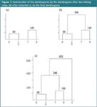
Figure 1: Construction of the dendrogram; (a) the dendrogram after two linking steps, (b) after reduction 3, (c) the final dendrogram.

Selection of Clusters

Suppose the analyst wants to use a set of three orthogonal CS. This can be achieved by sequentially cutting the highest links in the dendrogram (here the links at dissimilarities of 603 and 346). The clusters obtained are CS6 + CS10, CS7 + CS9 and CS3. The clustering appears logical since CS6 and CS10 are two silica-based stationary phases both run at pH 3. CS7 and CS9 are also silica-based but are run at pH values around 7 and the very differently behaving CS3 is zirconia-based. The chromatographer would select one CS out of each group (i.e., CS6 or CS10, CS7 or CS9, and CS3). The orthogonal set would, therefore, consist of two silica-based phases, with mobile phases of pH 3 and about pH 7 respectively, and a zirconia-based phase.

Conclusions

The mathematics employed in clustering is often very simple and this is certainly the situation for the algorithm described here. It can also be applied for the data analysis of the tables that would be obtained in the other instances described in the introduction, except that another (dis)similarity measure might be applied.

Many clustering methods are available and choosing the best for a given application and the proper dissimilarity measure requires some experience. The hierarchical agglomerative average linkage described here is the best known algorithm. The terms "hierarchical" and "average" were already explained previously. "Agglomerative" means that the method starts at the bottom of the tree and agglomerates individual objects and later small clusters into larger units. Divisive methods also exist but are seldom used. The whole set of objects is then first divided into smaller clusters, which are again divided until eventually all clusters contain only one object. Non-hierarchical methods are also used and, instead of average linkage, other types of linkage such as single linkage are possible. In the next column some of these alternatives will be described.

In many instances it is useful to apply both clustering and principal component analysis (PCA) to the same data sets.^3,4 An example can be found in references 5 and 6. The two methods are complementary: clustering offers a formal classification, while the visualization of the structure of the data set is often clearer with PCA.

Column editor Desire Luc Massart was an emeritus professor at the Vrije Universiteit Brussel, Belgium and performed research on chemometrics in process analysis and its use in the detection of counterfeiting products or illegal manufacturing processes. Johanna (An) Smeyers-Verbeke is a professor at the Vrije Universiteit Brussel and is head of the department of analytical chemistry and pharmaceutical technology. Yvan Vander Heyden is a professor at the same university and heads a research group on chemometrics and separation science.

References

1. D. L. Massart and Y. Vander Heyden, LCGC Eur., 17(9), 467–471 (2004).

2. E. Van Gyseghem et al., J. Chromatogr. A, 988, 77 (2003).

3. D. L. Massart and Y. Vander Heyden, LCGC Eur., 17(11), 586–591 (2004).

4. D. L. Massart and Y. Vander Heyden, LCGC Eur., 18(2), 84–89 (2005).

5. K. Le Mapihan, J. Vial and A. Jardy, J. of Chromatogr. A, 1088, 16–23 (2005).

6. K. Le Mapihan, J. Vial and A. Jardy, J. of Chromatogr. A, 1030, 135–147 (2004).