A Flash Qualitative Identification Method for the Specific Component in a Mixture Based on Diode Array Detector

This paper proposes a new method of flash qualitative identification (FQI) to qualitatively identify a certain target component from a mixture within half a second by disusing the analytical column, which is a time-consuming unit in current chromatography instruments. First, a Noised Spectrum Identification (NSI) model was constructed for the data set generated directly by diode array detector (DAD) without the process in an analytical column. Then, a method called vector error algorithm (VEA) was proposed to generate an error according to the DAD data set for a mixture and a specific spectrum for the target component to be identified. A criterion based on the error generated by the VEA is used to give a judgement of whether the specific spectrum exists in the DAD data set. Several simulations demonstrate the high performance of the FQI method, and an experiment for three known materials was carried out to validate the effectiveness of this method. The results show that the NSI model concurs with the real experiment result; therefore, the error generated by the VEA was an effective criterion to identify a specific component qualitatively, and the FQI method could finish the identification task within half a second.

Chromatography has been developed as a set of laboratory techniques that are widely applied in the quality control (QC) of mixtures such as herbal medicine, grape wine, petroleum, judicial expertise, and others. Chromatography is further classified as gas chromatography (GC) and liquid chromatography (LC) according to the mobile phase. With the development of the modern instrument, the ultrahigh-pressure LC (UHPLC) technique was born. High performance liquid chromatography (HPLC) is an important branch of chromatography. HPLC uses liquid as the mobile phase, and it employs a high-pressure infusion system to pump a single solvent with different polarities, or mixed solvents and buffers, in different proportions into the stationary phase. After the components in the column are separated, the chromatographic column enters the detector for detection to realize the analysis of the sample. Compared with HPLC, UHPLC has the advantages of higher resolution, faster speed, and greater sensitivity. Although the technique improves the speed, sensitivity, and resolution of HPLC, its original practicability and principle are retained. The significant advantage of UHPLC is that it can shorten the analysis time and improve work efficiency (for example, for a related substance analysis method, the use of HPLC to run a needle is 75 min; with UHPLC, this task can be completed in 10 min), and the analysis efficiency is increased by nearly 7.5 times. Of course, the analysis efficiency has been improved so much that the supporting equipment is certainly not for fun. UHPLC requires a small particle hybrid packing (1.7 μm) column, a higher pressure (up to 15000 psi), and a low system volume infusion unit. Although the supporting equipment can greatly shorten the analysis time depending on the complexity of the sample, it usually takes many minutes to complete the analysis process. To reduce the time consumed during the process of the chromatography, the diode array detector (DAD), combined with chemometrics methods such as evolving factor analysis (EFA) (1–3), multivariate curve resolution alternating least square (MCR-ALS) (4–7), the iterative algorithm (IA) (8,9), independent component analysis (ICA) (10,11), general reference curve measurement (GRCM) (12,13), and more, are introduced to pick chromatogram peaks from the raw data set generated by the hyphenated instrument of HPLC and DAD (14). The above methods could improve the resolution of the instruments, but they cannot reduce the time consumed during the chromatography process because it is influenced by the analytical column.

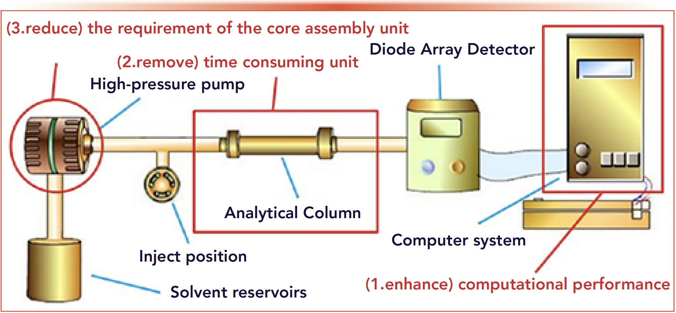
As shown in Figure 1, the analytical column is the time-consuming unit in a HPLC (or UHPLC) instrument. To further cut down the time used for an analysis process, this paper proposes a totally new software calculation method to qualitatively identify a specific component from a mixture within half second by disusing the analytical column. Because this method reduces the time for analysis sharply from 10–30 min down to around 200 ms, we call it the flash qualitative identification (FQI) method. Furthermore, the remove of the analytical column will reduce the requirement of the high-pressure pump.

FIGURE 1: Principle of the FQI method.

The remainder of this paper is arranged as follows: the principle of the FQI Method is introduced; the simulations and experiments to demonstrate the performance and practicability of this method are provided; and then we draw the conclusions from our study and propose future works.

The FQI Method

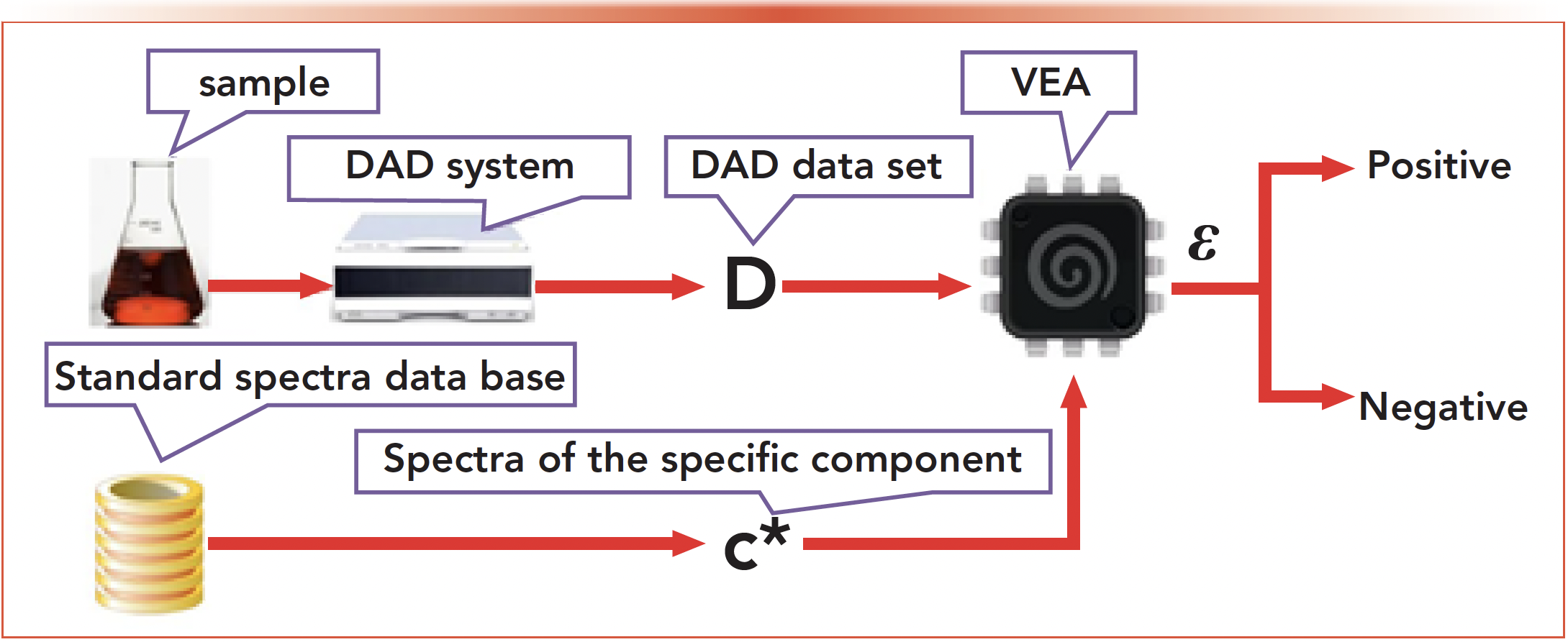
The operation process of the FQI method is demonstrated in Figure 2. First, the objective material for analysis is prepared to be a sample. Then, input the sample into the instrument to generate DAD data set D. On the other hand, the spectrum c* of the specific component to be identified is abstracted from the standard database. When the DAD data set D and the spectrum c* is inputted into the vector error algorithm (VEA), an error ɛ will be generated. Finally, the result of positive or negative could be given based on the error ɛ. The modeling for the DAD data set is introduced first; then, the design of the VEA will be explained carefully based on the DAD model.

FIGURE 2: The operation process of the flash qualitative identification algorithm.

Modelling for DAD Data Set

For component analysis, the model for HPLC-DAD data set as shown in equation 1 was used widely in many references (15,16)

where X is the HPLC-DAD data set with the dimension of w × t. The dimension w represents the wavelength, and the dimension t represents the sampling point along the retention time. a_i, i = 1,2,···, n are the column vectors indicating all the individual spectra. s^t/_i, i = 1,2,···, n are the row vectors indicating all the chromatogram peaks. The digital n is the number of the components contained in the data set X. The matrix N is the Gaussian noise. However, the model shown in equation 1 is not suitable for the research in this paper for the following two reasons, which are explained based on a simulated sample containing four components as shown in Figure 3.

FIGURE 3: Structure of the HPLC–DAD data set and DAD data set. (a) Chromatographic curves for components from column. (b) Spectra for components. (c) HPLC–DAD data set. (d) Chromatographic curves for components without the analytical column.

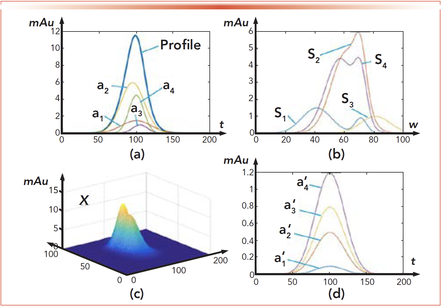
The first reason is because of the effect of the analytical column, the chromatographic peaks for different components express various values in width and peak position as shown in Figure 3a. Theoretically speaking, this feature makes the data set X = [a₁,a₂,a₃,a₄] × [s₁,s₂,s₃,s₄]^T, shown in Figure 3c, with the rank of four. However, if the analytical column was removed from the experimental system, the chromatographic peaks for all the components would share the same width and peak position as shown in Figure 3d according to the principle of the chromatography, which means the data set generated by X₁ = [a´₁,a´₂,a´₃,a´₄] × [s₁,s₂,s₃,s₄]^T, has the rank of one. Currently, there is no method could pick from a´₁ or s₁ from X₁. In Figure 3, the axis of mAu is the signal strength.

The algorithm proposed in our previous works based on equation 1 is to peak chromatogram peaks from s_i from X, and then to calculate spectra a_i based on s_i and X. In this paper, what we want to finish is to find a flash qualitative identification method for a specific component based on its spectrum. Therefore, the model shown in equation 1 is not suitable.

Based on the analysis above, the following noised spectrum identification (NSI) model is proposed.

where D is the DAD data set with the dimension of t × w. The dimension t represents the sampling point along the process time, and the dimension w represents the wavelength. p_i, i = 1,2,···, n are the column vectors indicating all individual chromatogram peaks. The vector p is a single peak curve to express the process for the mixture passing through the DAD instrument. c^t/_i, i = 1,2,···, n are the row vectors indicating all the spectra. The digital n is the number of the components contained in the data set D. The function ∙_i(p) adds different Gaussian noise to the vector p to generated vectors p_i.

The Design of VEA

Based the DAD model shown in equation 2 and the principle shown in Figure 2, following objective function is given.

where the vector w is unknown to construct vector y; the vector c* is the spectrum of the component which is going to be identified; the scalar of ɛ is the error between y and c*; the operator ||g||²₂ is the 2-norm of a vector; the note → means y looks like c* in shape. To solve equation 3, we rewrite it as

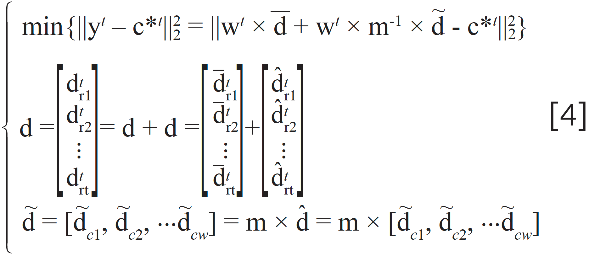
where d^t_ri, i = 1,2,···t are row vectors of matrix D; d^t_ri, i = 1,2,···t are row vectors, whose elements all equal to the mean value of d^t_ri, i = 1,2,···t; d^t_ri, i = 1,2,···t are row vectors after removing mean value from d^t_ri, i = 1,2,···t; the matrix D is transformed from the matrix D by a linear transformation, which makes the column vectors d^t_ci, i = 1,2,···w not correlated from each other and normalized as shown in equation 5. The method to obtain the matrix M is introduced in Appendix A.

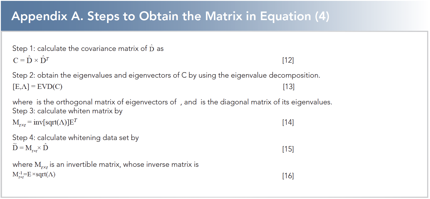
After analyzing equation 4, the term of w^T × ^–d equals to a constant vector, so equation 4 is reconstructed as

where d is a constant, and w is the number of the wavelength. Appendix B gives the reason why e{^~d*×^~d*^t} = w×i_(t+1)×(t+1).

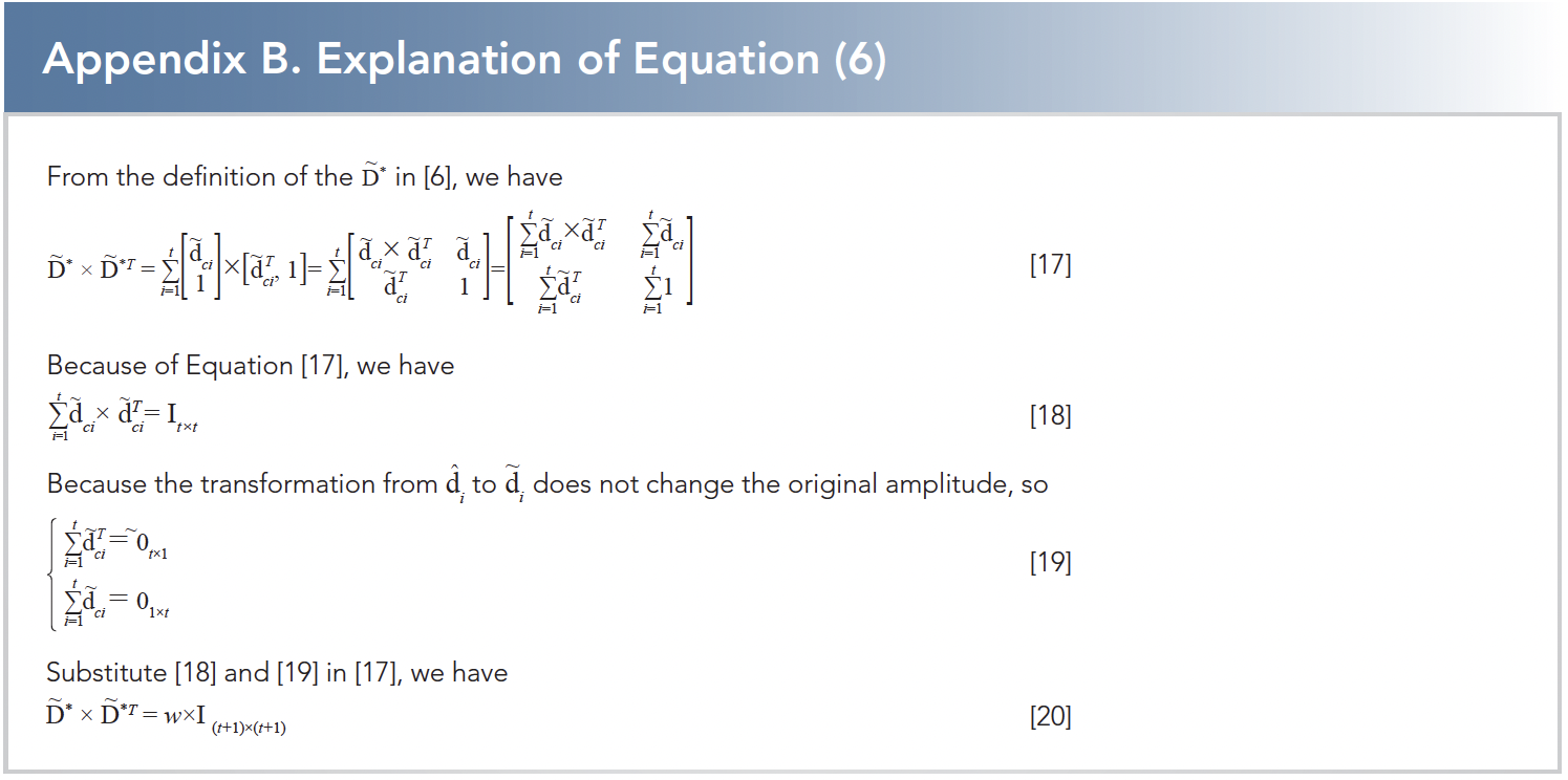
According to Karush-Kuhn-Tucher condition (17), the solution of equation 6 satisfies

where c*^T is the jth element in the vector c*^T. The Newton method (18) is adopted to solve equation 7, whose Jacobian matrix is calculated as

Then, the iteration for ^–b^t can be given as

Consequently, the curve of y^T can be calculated by the following equation.

Finally, the judgment for whether a specific component is contained in a mixture could be given by the criterion as shown in equation 11.

where the scalar value of ε* is a presetting small digital. Equation 3 is called the VEA. The scalar of ε is the output of VEA. Equation 11 is the criteria equation based on the VEA.

Simulations and Experiments

In this section, a group of simulations demonstrate the performance of the FQI method. On this basis, the minimum range of difference between target spectra and nontarget spectra is proved. Then, a data set, generated from HPLC-DAD instrument without passing through the analytical column, is calculated by the FQI method to indicate its effectiveness.

Simulations and Discussions

The simulation data set was generated by equation 2, where n is set to six. The vectors a´₁ shown in Figure 3d mixed with different level of Gaussian noise were selected as p₁ in equation 2. The vectors s₁ shown in Figure 3b mixed with different levels of Gaussian noise were selected as c₁ in equation 2.

For this study, 20 simulation data sets with different noise levels (SNR = 200, …, 30, 20, 10, 1) are generated equation 2. Four simulation data sets (SNR = 40, 20, 10, 1) are listed in this paper. As shown in Figure 4, 18 spectra curves are calculated by the FQI method, among which s_1-4 are known spectra contained in the data set D, and s_5-18 are spectra constructed different from s_1-4 in shape. The errors ε given by equation 3 for s_1-18 are listed in Table I.

FIGURE 4: 18 spectra for simulations S₁ through S₁₈.

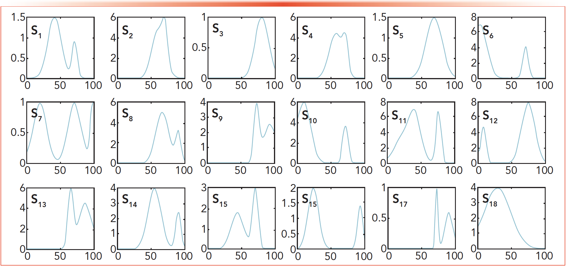
TABLE I: The results for the simulations

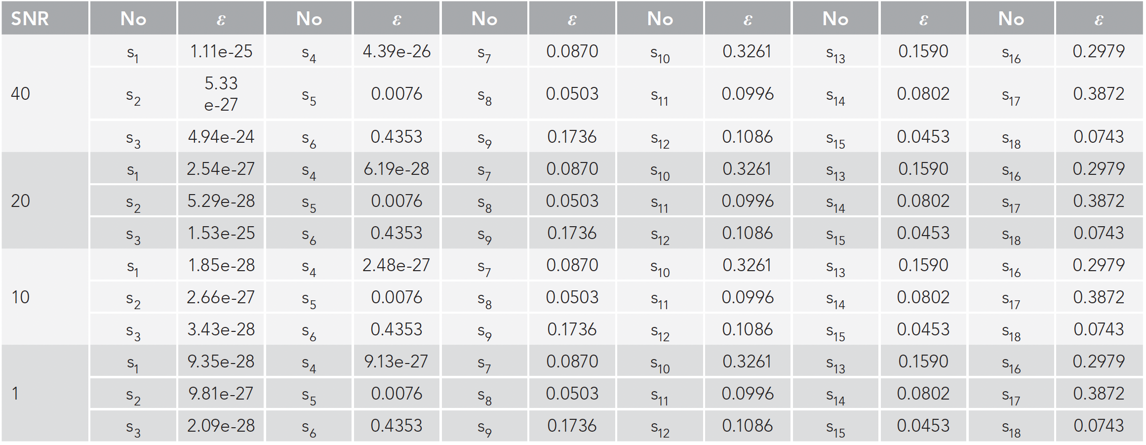
Among the 18 spectral curves, s₁ was selected as the experimental analysis object. As shown in Figure 5a, the eight curves changed in varying degrees on the basis of s₁ ∙ s²₁ is the overall offset of one unit on the basis of s₁, and s³₁ is the overall offset of two units on the basis of s₁ ∙ s⁴₁ - s⁹₁ is to change one of the 100 pixel points. Figure 5b is a graph of five distance formulas and corresponding errors for Euclidean distance, Mahalanobis distance, Chebyshev distance, chi-square distance, and Hamming distance. Among them, the red curve is Euclidean distance, Mahalanobis distance, and Chebyshev distance, these three curves coincide. Blue is chi-square distance and green is Hamming distance. We choose the Euclidean distance according to the experimental results. Table II lists the errors ε corresponding to the Euclidean distance of the nine deviation curve in Figure 5a. From the results, we can see:

FIGURE 5: Experimental diagram for distance: (a) s₁-based change graph, and (b) five deviation distance curve.

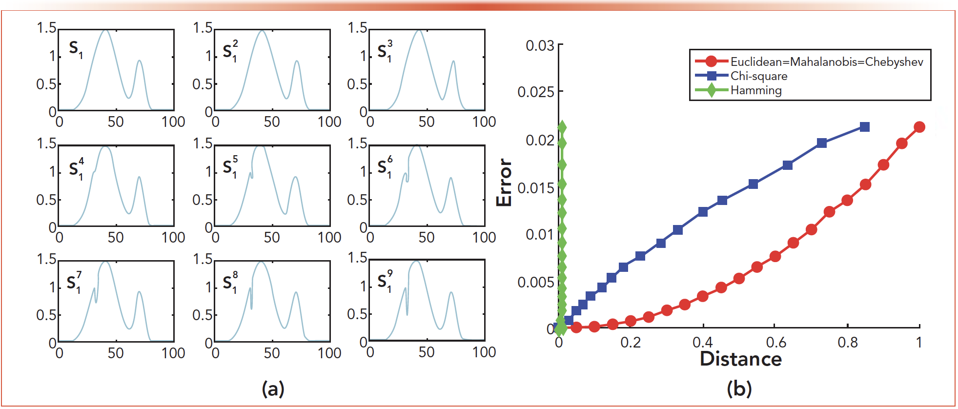
TABLE II: Error corresponding to deviation distance.

• The error ε calculated by the VEA is an effective criterion for judging whether a specific spectrum exists in the mixture and judge the similarity between them. In Table I, no matter how serious the noise existing in the data set is, the errors for the spectra of s_1-4 are always significantly smaller than those for s_5-18, which are different from s_1-4 in shape.
• Although four simulation data sets are generated by different noise levels, the final error results are almost the same. It can be seen from Table I that although the error of s_1-4 fluctuates, the error of s_5-18 does not change, which shows the experimental results are little affected by noise.
• The error ε calculated by the VEA is stable regardless of the noise level in the data set. In Table I, all errors calculated for s_5-18 are always the same although the noise levels are different. The differences among the errors for s_1-4 under various noise level may be caused by the calculation error of the computer.
• As can be seen from Table II, the greater the deviation distance, the greater the error. Our study found that the spectral curve allowed 0.3 offset distance. When Δ < 0.3, it is shown that the curve exists in the mixture, and when Δ > 0.3, the curve does not exist in the mixture.

Experiments and Discussions

The reference materials of C₆H₄SO₂NNaCO · 2H₂O (GBW (E) 100008, 1.00 mg/mL), C₄H₄KNO₄S (GBW (E) 1001711.00 mg/mL), C₆H₈O₂ (GBW (E) 100007, 1.00 mg/mL) were purchased from the National Institute of Metrology in China. Then, 0.5 mL of the abovementioned three materials were abstracted separately and mixed with water until the mixture had a volume of 10 mL. The chromatography instrument used was provided by Waters and equipped with a 2695 separating element, a 2998 DAD, and an Empower 3 workstation. The scan model is 3D with wavelength from 200 nm to 500 nm. The flow rate is set at 0.5 mL/min. The amount of the sample is selected as 10 μL.

Four DAD data sets of D,D₁,D₂,D₃ are generated by the instrument without the analytical column for the mixture, the C₆H₄SO₂NNaCO · 2H₂O, the C₄H₄KNO₄S, and the C₆H₈O₂ respectively. The time used for the individual experiment is only 0.2 s. And three spectra of s_1-3 can be abstracted for the three materials from D₁,D₂,D₃ in Figure 6. Similarly as the simulations, thirteen spectra of s_4-16, shown in Figure 7, are constructed based on s_1-3, which are different from s_1-3 in shape. We input the matrix D and the spectra s_1-16 into the VEA, the errors are shown in Figure 8 and Table III.

FIGURE 6: The DAD data sets and the spectra of the components.

FIGURE 7: The spectra for test set (s₁ through s₁₆).

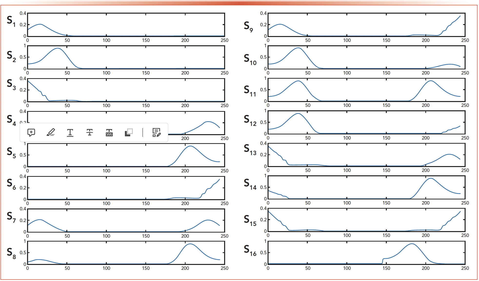
FIGURE 8: Error plot for the spectra.

TABLE III: The results for the simulations

Similar to the simulation experiment, we selected s₃ as the experimental analysis object in these 16 spectral curves. As shown in Figure 9a, s²₃ is the overall offset of one unit on the basis of s₃, and s³₃ is the overall offset of two units on the basis of s₃ ∙ s⁴₃ - s⁹₃ is to change one of the 244 pixel points. Figure 9b is a graph of the errors corresponding to the five deviation distances. Table IV lists the errors ε corresponding to the euclidean distance Δ of the nine deviation curve in Figure 9a. From the results, we can see:

FIGURE 9: Experimental diagram for distance: (a) s₃ based change graph. (b) Five deviation distance curve.

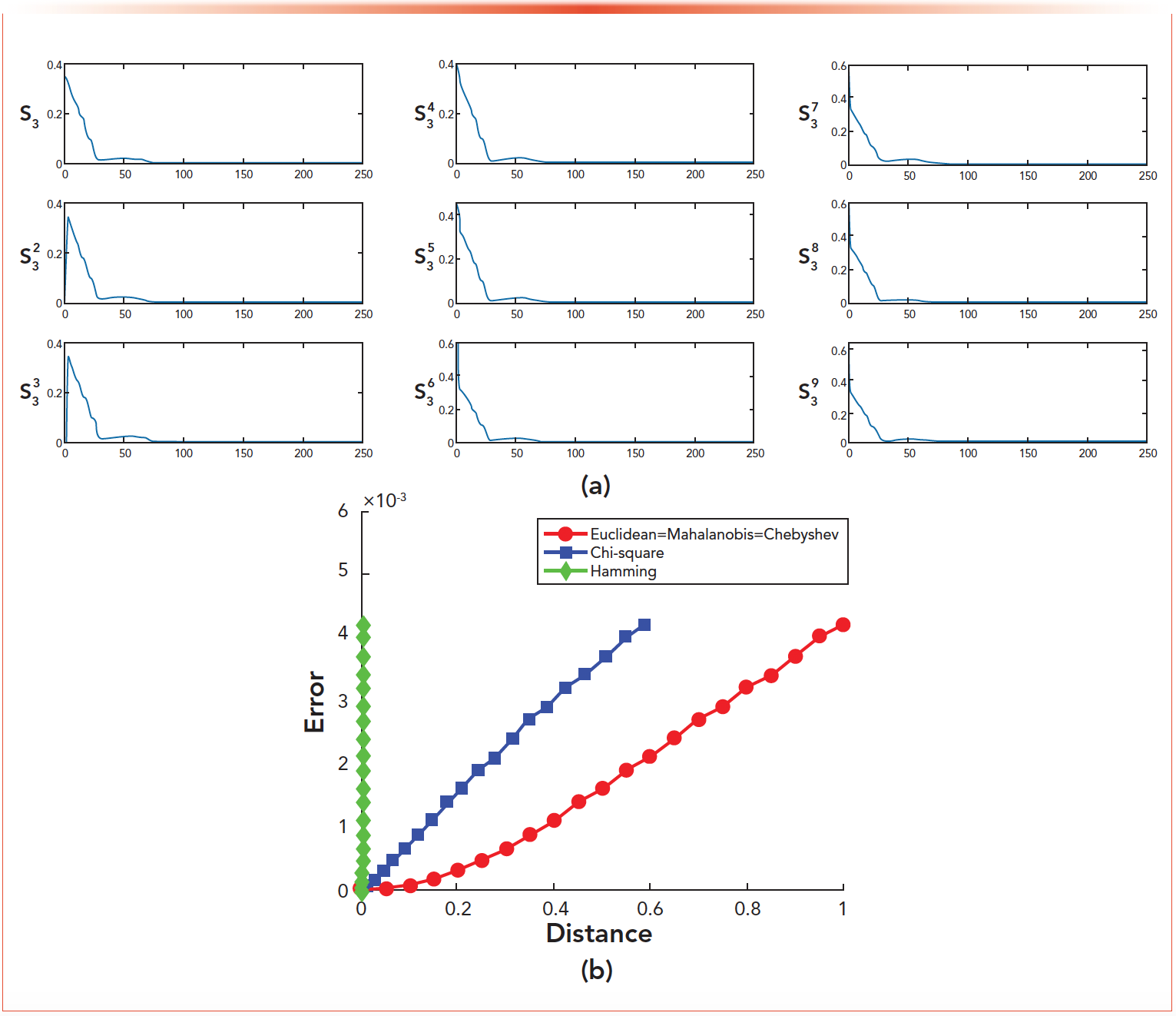
TABLE IV: Error corresponding to deviation distance

• The error calculated by the VEA could be used as a criterion to judge whether the mixture contain specific material represented by its spectrum. The size of the error is inversely proportional to whether the mixture contains the specific material represented by its spectrum. When the error is small enough or tends to be stable, it can be said that the mixture contains the specific material represented.
• It can be seen from Figures 7 and 8 that the errors for s_1-3 are smaller than those for s_4-16. The reason why the errors for s₁₀ and s₁₂ are close to those for s_1-3 is because the shape of s₁₀ and s₁₂ are close to the shape of s₂. However, the error of s₆ is the biggest because the shape difference between s₆ and s_1-3 is the biggest. This error shows that it is necessary to construct the curve according to the shape of the spectrum, and the similarity between the curve and the real spectrum determines its accurate value.
• The larger the amount of the material, the smaller the error calculated for its spectrum. In Table III, the error for s₂ is much smaller than those for s₁ and s₃. The reason could be that the amount of the material represented by s₂ is larger than those represented by s₁ and s₃. From Figure 7, the amplitude of s₂ is obviously bigger than those for s₁ and s₃.

Conclusions and Future Work

Conclusions

• A mathematical model named NSI for DAD data set was proposed in this paper. And based on this NSI model, a FQI method was proposed to identify a specific material from a mixture within half second. Through simulations and experiments, the method was proved to be effective and efficient in the qualitative identification for a specific material from a mixture.
• The gap between the errors given by the VEA for target spectra, such as s_1-4 in Figure 4, and non-target spectra, such as s_5-18 in Figure 4, is significant for simulations, whereas this gap for experiments is much smaller but still could be used as a criterion to finish the qualitative identification.
• The FQI method proposed in this paper did not need the analytical column in the instrument, and could finish the identification within a half second. This feature would bring a big change in the analytical research.

Future Work

• For experiments, how to enlarge the gap between errors for target spectra and non-target spectra will be researched in the near future, which will make the method more practical.
• For some application, the qualitative identification is not enough, so relative quantitative analytical method based on the FQI method should be proposed in the future, which could enhance the practicability of this method.

Acknowledgment

This work was supported in part by National Natural Science Foundation of China under Grant 61973105, Henan Natural Science Foundation under Grant 162300410125, Innovative Scientists and Technicians Team of Henan Provincial High Education (20IRTSTHN019), the Innovative Scientists and Technicians Team of Henan Polytechnic University (T2019-2), and the Henan Polytechnic University Doc Fund under Grant B2016-16.

References

(1) Zarghani, M.; Parastar, H. Joint Approximate Diagonalization of Eigenmatrices as a High-Throughput Approach for Analysis of Hyphenated and Comprehensive Two-Dimensional Gas Chromatographic Data. J. Chromatogr. A 2017, 1524, 188–201. DOI: 10.1016/j.chroma.2017.09.060

(2) Ghaheri, S.; Masoum, S.; Gholami, A. Resolving of Challenging Gas Chromatography–Mass Spectrometry Peak Clusters in Fragrance Samples Using Multicomponent Factorization Approaches Based on Polygon Inflation Algorithm. J. Chromatogr. A 2016, 1429, 317–328. DOI: 10.1016/j.chroma.2015.12.003

(3) Cook, D. W.; Oram, K. G.; Rutan, S. C.; Stoll, D. R. Rational Design of Mixtures for Chromatographic Peak Tracking Applications Via Multivariate Selectivity. Anal. Chim. Acta: X 2019, 2, 100010. DOI: 10.1016/j.acax.2019.100010

(4) Davis, J. M. Prediction by Statistical Overlap Theory of Fraction of Baseline Occupied by Chromatographic Peaks. J. Chromatogr. A 2021, 1640, 461931. DOI: 10.1016/j.chroma.2021.461931

(5) Ahmadvand, M.; Parastar, H.; Sereshti, H.; Olivieri, A.; Tauler, R. A Systematic Study on the Effect of Noise and Shift on Multivariate Figures of Merit of Second-Order Calibration Algorithms. Anal. Chim. Acta 2017, 952, 18–31. DOI: 10.1016/j.aca.2016.11.070

(6) Taheri, M.; Bagheri, M.; Moazeni-Pourasil, R. S.; Ghassempour, A. Response Surface Methodology Based on Central Composite Design Accompanied by Multivariate Curve Resolution to Model Gradient Hydrophilic Interaction Liquid Chromatography: Prediction of Separation for Five Major Opium Alkaloids. J. Sep. Sci. 2017, 40 (18), 3602–3611. DOI: 10.1002/jssc.201700416

(7) Dadashi, M.; Ghaffari, S.; Bakhtiari, A. R.; Tauler, R. Multivariate Curve Resolution of Organic Pollution Patterns in Mangrove Forest Sediment from Qeshm Island and Khamir Port-Persian Gulf, Iran. Environ. Sci. Pollut. Res. Int. 2018, 25, 723–735. DOI: 10.1007/s11356-017-0450-z

(8) Wahab, M. F.; Berthod, A.; Armstrong, D. W. Extending the Power Transform Approach for Recovering Areas of Overlapping Peaks. J. Sep. Sci. 2019, 42 (24), 3604–3610. DOI: 10.1002/jssc.201900799

(9) Davis, J. M. Theory of the Probability of Total Resolution in Chromatograms with Systematic Variation of Average Peak Spacing and Peak Width. J. Chromatogr. A 2019, 1588, 150–158. DOI: 10.1016/j.chroma.2018.12.031

(10) Hellinghausen, G.; Wahab, M. F.; Armstrong, D. W. Improving Peak Capacities Over 100 in Less Than 60 Seconds: Operating Above Normal Peak Capacity Limits with Signal Processing. Anal. Bioanal. Chem. 2020, 412, 1925–1932. DOI: 10.1007/s00216-020-02444-8

(11) Ciogli, A.; Ismail, O. H.; Mazzoccanti, G.; Villani, C.; Gasparrini, F. Enantioselective Ultra High Performance Liquid and Supercritical Fluid Chromatography: The Race to the Shortest Chromatogram. J. Sep. Sci. 2018, 41 (6), 1307–1318. DOI: 10.1002/jssc.201701406

(12) Cui, L.; Poon, J.; Poon, S. K.; et al. "An Improved Independent Component Analysis Model for 3D Chromatogram Separation and Its Solution by Multi-Areas Genetic Algorithm,” paper presented at the 2014 IEEE International Conference on Bioinformatics and Biomedicine, Shanghai, China, 2014.

(13) Cui, L.; Ling, Z.; Poon, J.; et al. Generalized Gaussian Reference Curve Measurement Model for High Performance Liquid Chromatography with Diode Array Detector Separation and Its Solution by Multi-Target Intermittent Particle Swarm Optimization. J. Chemom. 2015, 29 (3), 146–153. DOI: 10.1002/cem.2683

(14) De Luca, S.; Ciotoli, E.; Biancolillo, A.; et al. Simultaneous Quantification of Caffeine and Chlorogenic Acid in Coffee Green Beans and Varietal Classification of the Samples by HPLC-DAD Coupled with Chemometrics. Environ. Sci. Pollut. Res. 2018, 25, 28748–28759. DOI: 10.1007/s11356-018-1379-6

(15) Liu, Z.; Wu, H.- L.; Xie, L.- X.; et al. Direct and Interference-Free Determination of Thirteen Phenolic Compounds in Red Wines Using a Chemometrics-Assisted HPLC-DAD Strategy for Authentication of Vintage Year. Anal. Methods 2017, 9 (22), 3361–3374. DOI: 10.1039/C7AY00415J

(16) Yang, F.; Sun, G.; Chen, J. Development of a HPLC-DAD Method Combined with Multicomponent Chemometrics and Antioxidant Capacity to Monitor the Quality Consistency of Compound Bismuth Aluminate Tablets by Comprehensive Quantified Fingerprint Method. Anal. Methods 2017, 9 (27), 4082–4090. DOI: 10.1039/C7AY00916J

(17) Huang, X.- Y.; Pei, D.; Liu, J.- F.; Di, D.- L. A Review on Chiral Separation by Counter-Current Chromatography: Development, Applications and Future Outlook. J. Chromatogr. A 2018, 1531, 1–12. DOI: 10.1016/j.chroma.2017.10.073

(18) Müller, M.; Wasmer, K.; Vetter, W. Multiple Injection Mode With or Without Repeated Sample Injections: Strategies to Enhance Productivity in Countercurrent Chromatography. J. Chromatogr. A 2018, 1556, 88–96. DOI: 10.1016/j.chroma.2018.04.069

ABOUT THE AUTHORS

Lizhi Cui, Xuan Li, Zebin He, Yi Yang, Bingfeng Li, Keping Wang, Xinwei Li, Junqi Yang, and Xuhui Bu are with the School of Electrical Engineering and Automation at Henan Polytechnic University, in Henan, China.

Weina He is with the School of Computer at Pingdingshan University, in Henan, Pingdingshan, China.

Direct correspondence to Xuan Li at lixuan592021@163.com