Weighted Linear Least-Squares Fit — A Need? Monte Carlo Simulation Gives the Answer

Spreadsheet computer simulations can identify the influencing factors for the set-up of a calibration function such as the number of calibration points and their distribution or the position of the experimental points. A simple linear least-squares fit (linear regression) is not always allowed from theory but a weighted fit may be needed. By using a Monte Carlo approach, that is, by generating a large number of calibration functions and associated sample data points (for example 1000 for each set of simulations), the quality of the experimental results (bias and standard deviation) can be studied under different conditions. This article presents a spreadsheet for the simulation of unweighted and weighted linear least-squares fit. In practice, weighted fitting is only needed if all of the following conditions are fulfilled: a large calibration range; an equal distribution of the calibration points; the absolute standard deviations of the calibration points are not constant; and a sample result is at the lower end of the calibration range.

Photo Credit: Andrey Prokhorov/Getty Images

Quantitative chromatographic methods require calibration by a pure standard that is identical to the analyte. Single-point calibration is quick and can be used if the analyst was able to show during validation that the relation between analyte concentration and signal (peak area or height) is linear and that a blank sample gives a signal value of zero. However, in many real laboratory situations a multipoint calibration is used. Several standard solutions of well-known analyte concentration x_standard are investigated by the analytical instrument, yielding their corresponding signals y_standard. The calibration function

with a = intercept and b = slope is calculated by linear least-squares fit (also called linear regression) with three or more calibration points (1–5). The sample is subsequently investigated, yielding its signal y_sample, and the analysis function is used to calculate the analytical result; namely the concentration (c) of the analyte in the prepared sample solution (which in most cases is not the analyte concentration in the sample proper because the latter was prepared, diluted etc.):

In common laboratory situations, the x_standard and y_standard values usually differ in their "quality", which is expressed as standard deviation or uncertainty. The standard will be very pure and, at its best, come with a certificate of analysis; it will be weighed and diluted with great care. Therefore the analyte concentrations of the standard solutions are known with low uncertainty, for example in the 10^–3 (0.1%) range or even better (6). (The uncommon case of noteworthy uncertainty of the x data was discussed by Tellinghuisen [7].)

In contrast to such precision, the y_standard values may have a higher uncertainty. This is because it is difficult to keep the injection precision of a liquid chromatograph at ≤1% in the long term (8); the analytical process may have its own variability; and the signal-to-noise ratio (S/N) of the signal adds significantly to the repeatability of the signal if S/N is smaller than 100 (9). Moreover, the classical model of linear least-squares fit works with exactly known x_standard values and a constant absolute standard deviation of all y_standard points (1).

The analyst should try to set up a calibration function that yields analytical results with low standard deviation and bias while keeping in mind that the laboratory workload increases with the number of calibration points. Questions of interest are:

• Is a weighted fit needed or not?

• How many calibration points are necessary?

• How should the calibration points be distributed?

• Is a narrow calibration interval better than a wide one?

• Where should the calibration function be placed with regard to the expected or possible analytical result?

It is instructive to find the answers to these questions by simulation. This article demonstrates how weighted fits can be simulated with spreadsheet calculations (by using random numbers). Unweighted fits are also calculated by the spreadsheet, and can evaluate if the complicated weighting process is really required. By using a Monte Carlo approach, the n-fold repetition of the simulation (here n = 1000) is possible, therefore showing the mean of the x_sample result, its bias from the theoretically true value, and the standard deviation that can be expected.

Simulation Set-Up

Simulations of calibration functions and experimental data can be performed with Excel software. The order of magnitude of the y_standard data shown in this paper is 10 times larger than that of the corresponding x_standard data to obtain a clear distinction. The x_standard values have no uncertainty, as explained above. The y values, which represent peak areas or heights, achieved a normally distributed (or Gauss) standard deviation, either with a constant absolute standard deviation (SD) (simple linear least-squares fit) or with a constant relative standard deviation (RSD) (weighted linear least-squares fit).

Although it would be possible to use the random number generator of Excel for this purpose, this approach is inferior because it is based on an unknown algorithm and therefore the generated numbers are not really random in nature. Numbers with genuine randomness are to be preferred; they can be obtained from the free website www.random.org, which generates the required numbers from atmospheric noise. Their number, type of distribution (Gauss for this study), mean, standard deviation, and number of significant digits can be selected. A possible set of random numbers shown here has a mean of 50,000, a standard deviation of 5000, five digits, and a size of 1000 numbers - all formatted into one column. These 1000 data points can be directly pasted in a single operation from the website into a column of the spreadsheet.

The spreadsheet discussed here is based on five calibration points. A simulation procedure runs as follows:

• 5 × 1000 calibration points with fixed x values and scattering y values (from www.random.org, select FREE services Numbers, Gaussian Generator), 10 times larger than the corresponding x values, are put into columns A–E of an Excel spreadsheet.

• The calibration function is calculated by either simple or weighted linear least-squares fit. In the case described above, its slope is about 10 because y = 10x.

• 1000 y_sample values, located within the range of y_standard values and with a defined SD or RSD, are taken from www.random.org, put into column F, and the corresponding x_sample values calculated using the calibration function generated before, once in the unweighted (usual) mode and once by weighting.

To summarize: The scatter of the calculated mean x_sample value is the result of the scatter of the 1000 calibration functions and of the corresponding 1000 y_sample values. This kind of simulation is a Monte Carlo approach (10–15). The data of interest is not found with a closed mathematical function or by an iterative procedure but by the repeated calculation of the possible result under varying starting conditions. In this article, the variations have a normal (Gauss) distribution with a defined and selected SD or RSD. Depending on the problem, that is, the number and complexity of the involved calculations, a Monte Carlo process should include a great number of simulations. For the issues discussed here 1000 simulations give x_sample RSDs that are stable at two figures, such as 4.3%, but not at three figures; from one 1000-simulations-set to another, the result may differ in the second decimal place, for example 4.28% and 4.34%. It can be assumed that 10⁴ simulations are necessary for two stable decimal places, but in chemical analyses such excessive precision is usually not needed. It is up to the user to check this problem and to expand the number of runs, if necessary, up to 10⁵. If weighted linear least-squares fit is needed (see below), the accuracy (bias) of the x_sample value can be of greater importance than its precision.

The Simple Case: y Data with Constant Standard Deviation

The simple linear fitting of x–y data, that is, ordinary least-squares (1–4), is based on two prerequisites. Firstly, the x data have no scatter, only the y data have, as explained and justified above. Secondly, the scatter of the y data is constant; all y values have the same absolute SD irrespective of their value. This second prerequisite is known as homoscedasticity (16). It will occur if an autosampler works with a constant standard deviation, such as 1 μL, irrespective of the injected volume, and if the calibration points are generated with different volumes of the same solution (instead of the same volume of several solutions with different concentrations).

Obviously, it is not difficult to set up a spreadsheet for the calculation of a linear least-squares fit if the data is homoscedastic. The Excel commands for SLOPE and INTERCEPT are available on demand. Such a spreadsheet can be of great didactic value because it allows many aspects to be studied:

How Many Calibration Points Are Needed? Simulations show that the precision of the analytical result increases (SD decreases) with increasing number of points (data not shown here).

Is a Narrow Calibration Range Advantageous? No, the range of calibration has no influence on the precision of the analytical result as long as its position remains unchanged, for example in the middle of the range (data not shown here). However, it is questionable if the absolute SD of the y values is constant in real situations. Can we expect an experimental SD of 100 if y = 500 and also if y = 10,000? It is an advantage that such set-ups can be studied in advance by Monte Carlo simulations.

Where is the Best Position of the Sample Signal? The scatter of the analytical result x_sample has two influencing factors: the scatter of the position of the calibration line and the scatter of the measured signal y_sample. Since the SD of all signals in the Simple Case is constant, this number affects a low y_sample much more than a high one. Even without simulation, it is no surprise that under these circumstances, the best position of the sample signal is at the upper end of the calibration function.

Does an Irregular Distribution of the Calibration Points Make Sense? Researchers frequently want "to kill two birds with one stone" and place more calibration points at low concentrations than at high ones. However, simulations with constant SDs of the y_standard points show that an irregular distribution has practically no influence on the result (data not shown here).

Does a Repeat Determination (Double Determination) Make Sense? Some analysts perform a second, repeat measurement in the hope of obtaining a more reliable result. This approach is maybe a good idea, maybe not. In routine quality control, it is best to observe the analytical performance by control charts (17). If the method is under statistical control, that is, if the analysis of a reference material with constant properties yields constant results of accepted standard deviation, then one can trust the result of a single determination. If these preconditions are not fulfilled (in non-routine analysis for example), more than one analysis should be performed. It is then necessary to do at least two analyses from scratch by taking two samples, making individual sample preparations (preferably not in parallel but on different days), leading to individual measurements and to individual results. However, it is not good practice to simply analyze the final sample solution two or three times. Such a procedure yields nothing more than the repeatability of the instrument, which has nothing to do with the repeatability of the sample preparation or the inhomogeneity of the sample. This kind of "repeat determination" cannot be recommended. In addition, it is a matter of course that the analytical instrument should work with higher precision (lower SD) than the observed, "true" SD of the samples (18). Despite these concerns, the influence of a second analysis can be studied with a spreadsheet.

Other Simulation Possibilities:

• Several calibration points of the same x_standard value that results in a calibration with 3 × 5 = 15 points, for example.

• Simulations with constant SD of the y_standard points and another SD of y_sample.

• The influence of wrong calibration points, for example, resulting from wrong weighing or wrong dilution.

The Difficult Case: y Data with Variable Standard Deviation (or Constant Relative Standard Deviation as a Special Case)

A common situation in analytical chemistry is the constant (or nearly constant) RSD of the y values (the peak areas or heights). This happens if the autosampler works with a constant RSD of 1% or similar, irrespective of the absolute injected volume. In such a case, the SDs of the calibration points are heteroscedastic (19) and one prerequisite for simple linear least-squares fit is no longer fulfilled. It must be replaced by the markedly more complicated weighted linear least-squares fit (20). Contemporary software packages for chromatographs come with tools for this procedure, but without disclosure of the algorithms used. Programmes for weighted linear least-squares fit have been proposed (21–23) and Tellinghuisen studied the problem with Monte Carlo computations (24–25). Kuss presented his approach in detail, not only in LCGC Europe (23) but also in a book with accompanying CD-ROM (26). This disk contains an Excel spreadsheet for weighted linear least-squares fit. The following discussion in this section is based on the Kuss spreadsheet; however, what is calculated by Kuss in rows is presented here in columns so that the 1000 simulations appear one below the other. As a consequence, the "weighted" Monte Carlo spreadsheet with five calibration points has approximately 50 columns and more than 1000 rows (Figure 1).

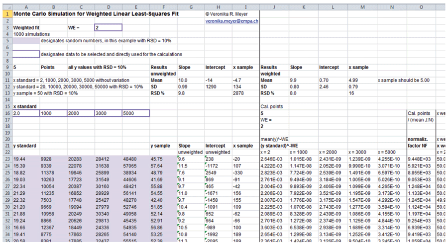
Figure 1: Example of an Excel spreadsheet for a 5-point weighted linear least-squares fit. It is 53 columns and 1022 rows. The first 12 simulations of 1000 are shown. All y_standard and y_sample values are random numbers (coloured cells). All data in a row are linked together, and an x_sample value is calculated from the data in its row. The mean of all 1000 weighted x_sample is 4.99 in this example; its true value is 5.00. The relative standard deviation (RSD) of the calibration function's intercept is not calculated because this information is not useful: the mean of the 1000 intercepts is close to 0 (remember that the y axis runs from 0 to 50,000), which would result in an absurd RSD.

Weighted Linear Least-Squares Fit: If all y RSDs are identical, for example 10%, the values at the upper end of the calibration get too much weight in a classical linear least-squares fit; the SD of y = 50,000 is 5000 while the SD of y = 1000 is only 100. As a consequence, the calibration function can be at the incorrect position in the lower range of the line (Figure 2). Therefore these SDs must be normalized or weighted with the factor WF = 1/y^WE. For an unweighted fit WF is 1/y, in the case of constant RSDs it is 1/y². In reality, the weighting exponent (WE) can be between 1 and > 2 because the SDs are potentially not generated by the autosampler alone. The WE can be determined by investigating the SDs of the highest and the lowest calibration points, which is a pragmatic approach to this problem (instead of studying the SDs of all calibration points).

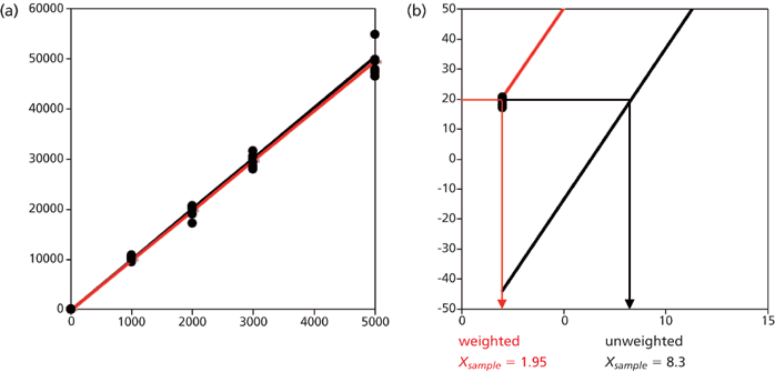
Figure 2: An example where a weighted fit is needed. The calibration range runs from x_standard = 2- 5000. The unweighted (black) and weighted (red) functions were obtained with 1000 simulations with all y_standard points having RSD = 10%, but the graph shows only six calibration points per concentration (partially covered by each other). (a): Full calibration range. (b): The lowermost part of the range, showing that the unweighted function would yield incorrect analytical results.

In ordinary least-squares fitting, the calibration function runs through the centroid, which is the point x(withbar),Ó¯, and is the means of the x_standard and y_standard values. In weighted least-squares fitting, the centroid is at x(withbar)_weighted, Ó¯_weighted. The slope of the function is:

and the intercept:

Calculation of the Weighting Exponent WE: The weighting exponent can be calculated pragmatically as follows (23,26):

with s = standard deviation, y(high) = highest y_standard value (mean), and y(low) = lowest y_standard value (mean).

This procedure can also be performed stepwise in a spreadsheet:

• Determine the (absolute) SDs of the lowest and the highest calibration points by multiple measurements of y_standard at these positions.

• Calculate the quotient of the squared SDs and its logarithm.

• Calculate the logarithms of both y_standard SDs and their difference.

• Calculate the quotient of the values obtained in step 2 and 3.

With constant RSD at y(high) and y(low), WE has the value of 2, irrespective of the percentage of the RSD. With constant SD at y(high) and y(low), WE = 0 and y^WE = 1, this is the unweighted case as discussed above. The experimental y_standard values of real analytical problems usually result in 0 < WE < 2. However, if the RSD at y_high is larger than the RSD at y_low (probably a very rare case), WE is higher than 2.

With a limited database it is not possible to know if y_high really has a large RSD (or if y_low has a small RSD) or if this result was obtained by chance. As an example, if all of the y_standard points have an RSD of 10%, the measured data at y_high may be 4500, 4529, and 5399, giving a RSD_y(high) = 10.6%. The y_low points may be 4.732, 4.877, and 5.369, giving a RSD_y(low) = 6.7%. In this case, WE = 2.3 instead of 2.0. The problem arises from the fact that 3 experiments are not sufficient to obtain a robust, "true" SD or RSD (27). However, the influence of WE on the analytical result must not be over-estimated. Usually it is small, as can be demonstrated by changing the exponent in the spreadsheet for weighted fit.

Weighted Linear Least-Squares Fit With a Spreadsheet: The set-up of the spreadsheet was explained in detail by Kuss (23). It concludes with the calculations of slope b and intercept a as illustrated in equations [3] and [4]. It handles not only weighting operations but also needs normalizations. The normalization factor (NF) is:

Calibration points are counted n-fold if a certain concentration is investigated n times; for example six different concentrations x_standard, analyzed twice each, gives 12 calibration points. The WE is calculated with a separate spreadsheet or is selected from experience (or from curiosity to study its influence). Table 1 presents the operations performed in the different columns of the spreadsheet discussed here; in rows 23 to 1022 the 1000 simulations are performed (not shown). Columns A–I calculate the unweighted case; the (long) part for the weighted case stretches over columns J–BA. With less than five calibration points, the spreadsheet would have less columns; with more points it would be larger (with six points nine more columns are needed, with seven points 18 more columns).

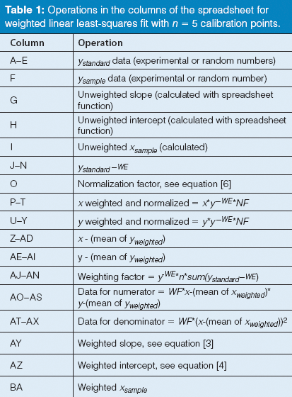
Table 1: Operations in the columns of the spreadsheet for weighted linear least-squares fit with n = 5 calibration points.

The spreadsheet for unweighted and weighted fit, investigated by Monte Carlo simulations, is available from the author on request for free (veronika.meyer@empa.ch or VRMeyer@bluewin.ch).

Under What Conditions is Weighting Needed?

The most interesting question in this context is of course: Under which circumstances is it necessary to perform the complicated process of a weighted fit?

Influence of the Calibration Range: Tellinghuisen found for the case where WE = 2 that weighting is not really needed if y_sample is in the middle of the calibration range, but that it is necessary for data at the lower end of the range (24). Monte Carlo simulations, always with 1000 runs, confirm this result. The wider the calibration range (for example three orders of magnitude), the more important weighting for low y_sample data is (Figure 2). In this example, a value at the lower end of y_sample = 20 results in a grossly erroneous x_sample of 8.3 in the unweighted case; the correct result should be 2.0. The weighted function with WE = 2 (because the RSDs of y_standard are constant at 10%) gives an astonishingly accurate x_sample of 1.95. In the middle of the calibration range, at y_sample = 30,000, it does not matter if the weighted or the unweighted function is used; x_sample is 2980 or 3030, respectively (should be 3000). The same situation is found at the upper end, namely x_sample = 4960 or 5050, respectively (should be 5000).

If the calibration range is narrow, the question "to weight or not?" has no clear answer. The 5-point, 10% RSD case of x_standard = 10, 20, 30, 40, and 50 and y_standard = 100, 200, 300, 400, and 500 (less than 1 order of magnitude) was studied with 1000 simulations each for y_sample points at different positions. At the lower end of the function, with y_sample = 100, the mean result for x_sample was 10.0 unweighted and 10.2 weighted (true value = 10.0). However, the RSD of x_sample was 19% unweighted vs. 12% weighted. Weighting gave a mean (of 1000 simulations) with some small bias but better precision. In the middle and at the upper end (y_sample = 250 and 500, respectively), the bias was also smaller in the unweighted case (x_sample = 25.1 and 50.6) than in the weighted one (x_sample = 25.4 and 51.2) and the precision was comparable in all four cases (11.3%, 11.7%, 12.5%, and 11.4%).

Unequal Distribution of the Calibration Points: When considering these results, there is one question still unanswered: Is weighting needed for a wide calibration range with four points at the lower end and one single at the upper end? This was studied with x_standard = 10, 20, 30, 40, and 5000 and corresponding y_standard values 10 times higher - all y values with RSD = 10%. The simulations show that weighting is not necessary, not even when the analytical result is at the lowest end (x_sample = 9.84 unweighted vs. 10.14 weighted; should be 10.0). Precision, however, is worse (higher RSD) with the simple fit (RSD x_sample = 24% vs. 12% at low end, 14% vs. 11% in the middle, 15% vs. 11% at high end). Analogous results are found when x_sample is in the middle of the range or at its upper end.

In the inverse situation, one single calibration point at the lower end and four at the upper end (probably a very rare situation), weighting is necessary if x_sample is at the lower end (data not shown here).

Recommendations for Weighting: These simulations lead to the conclusion that weighting is only needed if the SD of the calibration points is not constant; if the calibration range is large; if the calibration points are equally distributed; and if the analytical result is at the lower end of this range.

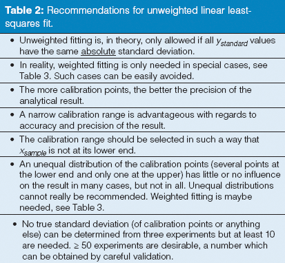
Table 2: Recommendations for unweighted linear least-squares fit.

Conclusions

Monte Carlo simulations allow different scenarios of calibration to be replicated to look for the best conditions for precision and bias. They can be performed with Excel software. Weighted fitting is necessary if the absolute SD of the y_standard points is not constant; if the calibration range is wide and with equally distributed points; and if the analytical result is at the lower end of the calibration function. Although the option of weighting is usually offered by the chromatographic data processing software, it can be wise to avoid such situations by working with narrow calibration ranges: Does it really make sense to establish a wide calibration range if you are only interested in the lowest concentrations? If you decide that weighting is needed, the selection of the weighting exponent is still open, and it should be chosen after the validation of the method. Table 2 and Table 3 summarize the unweighted and the weighted linear least-squares fit recommendations.

Table 3: Recommendations for weighted linear least-squares fit.

Veronika R. Meyer has a PhD in chemistry. She is a senior scientist at EMPA St. Gallen and a lecturer at the University of Bern, Bern, Switzerland (due to retire in 2015). Her scientific interests lie in chromatography, mainly in HPLC, and chemical metrology such as measurement uncertainty and validation. Her non-professional passions are mountaineering, reading, writing, and politics.

References

(1) D.S. Hage and J.D. Carr, Analytical Chemistry and Quantitative Analysis (Prentice Hall, Boston, Massachusetts, USA, 2011).

(2) J.N. Miller and J.C. Miller, Statistics and Chemometrics for Analytical Chemistry (Prentice Hall, Harlow, England, 6th edition, 2010), Chapter 5.

(3) S. Burke, LCGC Europe On-line Supplement, https://www.webdepot.umontreal.ca/Usagers/sauves/MonDepotPublic/CHM%203103/LCGC%20Eur%20Burke%202001%20-%202%20de%204.pdf (accessed December 2014).

(4) V. Barwick, Preparation of Calibration Curves - A Guide to Best Practice, LGC Ltd., 2003, http://www.lgcgroup.com/LGCGroup/media/PDFs/Our%20science/NMI%20landing%20page/Publications%20and%20resources/Guides/Calibration-curve-guide.pdf (accessed December 2014).

(5) J.J. Harynuk and J. Lam, J. Chem. Educ.86, 879 (2009).

(6) EURACHEM/CITAC Guide Quantifying Uncertainty in Analytical Measurement, 3rd ed. 2012, Example A1, http://eurachem.org/index.php/publications/guides/quam (accessed December 2014).

(7) J. Tellinghuisen, Analyst135, 1961–1969 (2010).

(8) S. Küppers, B. Renger, and V.R. Meyer, LCGC Europe13, 114–118 (2000).

(9) C. Meyer, P. Seiler, C. Bies, C. Cianculli, H. Wätzig, and V.R. Meyer, Electrophoresis33, 1509–1516 (2012).

(10) M. Chang, Monte Carlo Simulation for the Pharmaceutical Industry: Concepts, Algorithms, and Case Studies (CRC, Boca Raton, Florida, USA, 2011).

(11) J.L. Burrows, J. Pharm. Biomed. Anal.11, 523–531 (1993).

(12) J. Burrows, Bioanalysis5, 935–943 (2013).

(13) J. Burrows, Bioanalysis5, 945–958 (2013).

(14) J. Burrows, Bioanalysis5, 959–978 (2013).

(15) Joint Committee for Guides in Metrology, Evaluation of Measurement Data - Supplement 1 to the "Guide to the Expression of Uncertainty in Measurement" - Propagation of Distributions Using a Monte Carlo Method, 2008, http://www.bipm.org/utils/common/documents/jcgm/JCGM_101_2008_E.pdf (accessed December 2014).

(16) http://www.wikipedia.org/wiki/Homoscedasticity (accessed December 2014).

(17) E. Mullins, Analyst124, 433–442 (1999).

(18) B. Renger, J. Chromatogr. B745, 167–176 (2000).

(19) http://www.wikipedia.org/wiki/Heteroscedasticity (accessed December 2014).

(20) J.N. Miller, Analyst116, 3–14 (1991).

(21) M. Davidian and P.D. Haaland, Chemometr. Intell. Lab. Syst.9, 231–248 (1990).

(22) E.A. Desimoni, Analyst124, 1191–1196 (1999).

(23) H.J. Kuss, LCGC Europe16, 819–823 (2003).

(24) J. Tellinghuisen, Analyst132, 536–543 (2007).

(25) J. Tellinghuisen, J. Chromatogr. B 872, 162–166 (2008).

(26) H.J. Kuss, in Quantification in LC and GC - A Practical Guide to Good Chromatographic Data, H.J. Kuss and S. Kromidas, Eds. (Wiley-VCH, Weinheim, Germany, 2009), pp. 161–165.

(27) V.R. Meyer, LCGC Europe25(8), 417–424 (2012).