Screening Designs (Part 2) Data Analysis

Screening for important factors during method optimization or robustness testing usually involves two-level screening designs, such as fractional factorial and Plackett–Burman designs.¹ These designs allow evaluating the effects of a relatively high number of factors f on a response in a relatively small number of experiments (N ≥ f+1).

Part 1,² described these designs and related concepts, such as aliases, generators, design resolution, defining relations, contrast coefficients, interaction effects and confounding of effects. Part 2 will discuss the experimental protocol and the data analysis of a screening design approach.

Experimental Protocol

After selecting the factors and the experimental design, the experiments to execute are defined by replacing the design levels (– 1 and +1, occasionally 0) by the real factor levels. They are then executed and for each experiment the relevant response(s) are determined.

To minimize uncontrolled influences on the estimated factor effects, it is often recommended that the design experiments are executed in a random sequence.³ However, randomizing the experimental sequence will not always solve the problem, as will be discussed in the section on "occurrence of time effects".

Although it is not advisable for practical reasons experiments are sometimes blocked or sorted by one or more factors.³ In these situations, all experiments at one level of the factor are initially executed, followed by all at the others. Examples in chromatography can be found when, for instance, two columns are examined in a design or when the factor column temperature is considered.

Data Analysis

Calculation of effects: After performing the design experiments, the factor effects can be estimated by equation 1, as discussed in Part 1:

where ΣY(+1) and ΣY(–1) represent the sums of the responses where factor X is at (+1) and (–1) level, respectively, and N is the number of design experiments. Sometimes, normalized effects (Equation 2) are calculated.³ They are calculated relative to the average nominal result (Y-mean = Y-mean nominal) or the average design result (Y-mean = Y-mean_N).

Graphically, a bar plot (Figure 1) can be drawn, where the estimated factor effects are represented. When a statistical interpretation of the estimated effects is also performed, the critical effect (see further) can also be presented on this plot by horizontal lines.

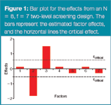
Figure 1

Many software packages present the result as a Pareto chart (Figure 2). In these plots, the absolute values of the effects are plotted. In many instances not the estimated effects are plotted but the so-called standardized effects, which are in fact the t-values (see further), obtained in the statistical interpretation. The critical effect is also drawn on this plot.

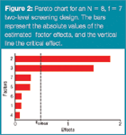
Figure 2

Alternatively, instead of effects, the coefficients of multiple regression analysis are sometimes reported. From these coefficients (b_x = b₁, b₂, ..., b_n), the corresponding factor effects (E_X = E₁, E₂, ..., E_n) can easily be calculated (Equation 3). Effects reflect the change in response between the levels (–1,+1) of a factor, while coefficients do between (0,+1), which explains the difference between both.⁴

When applying a three-level screening design (see Part 1), the effects between the levels (–1,0), (0,+1) and (–1,+1) can be estimated. For a reflected two-level design to screen the factors at three levels, the effects between (–1,0) and (0,+1) are calculated.

Graphical/statistical interpretation of effects: To evaluate the significance of the estimated factor effects, that is, to determine whether they are different from zero, they can be interpreted graphically and/or statistically.

Graphically, normal or half-normal probability plots can be drawn (Figure 3). In these plots, the non-significant effects are situated on a straight line through zero, while the significant deviate from it. However, occasionally it is not so evident to visually determine the important effects straightforwardly from these plots and therefore, in our opinion, it is recommended to combine the graphical with a statistical interpretation.

Figure 3

Statistical interpretation methods most frequently apply a t-test, in which the t-test statistic (Equation 4) is calculated as:

The t-value is based on the effect of a factor, E_X, and on the estimation of the standard error of an effect, (SE)_e. It is compared with a (tabulated) critical t-value, t_critical, which depends on the number of degrees of freedom associated with (SE)_e and usually determined at significance level α = 0.05. Equation 4 can be transformed so that a critical effect, E_critical, is computed (Equation 5) based on t_critical and (SE)_e.

An effect is significant when its t-value is larger than or equal to t_critical, or when its effect is in absolute value larger than or equal to E_critical. The error estimate (SE)_e can be determined in different ways, for instance from the variance of replicated experiments, from a priori declared negligible effects or from a posteriori defined negligible effects.

The first possibility is to derive (SE)_e from the variance of replicated experiments, s² , with (Equation 6), where n is the number of experiments performed at each factor level.

Either the variance of R replicates at nominal or centre point level, or the variance of duplicated design experiments

with d_i the difference between the duplicated experiments, can be used, with n equal to N/2 and N, respectively, and the number of degrees of freedom for t_critical R–1 and N, respectively. A requirement is that the replicates are measured at intermediate precision conditions and not under repeatability conditions (which is often the situation), because in the latter situation an underestimation of E_critical occurs, leading to a high number of erroneously considered significant effects. Another recommendation is that at least three degrees of freedom for t_critical should be available; that is, enough replicates are considered to estimate (SE)_e.

Second, (SE)_e can be derived from n_N a priori declared negligible effects, E_N, such as certain interaction or dummy factor effects in fractional factorial and Plackett–Burman designs, respectively (Equation 7). Here, it is recommended that at least three negligible effects are used to estimate (SE)_e. In robustness testing, two-factor interactions and dummy effects can usually be considered negligible. In method optimization, where the examined factor ranges are broader and thus effects larger, two-factor interactions are not always negligible and for the same reason, dummy factor effects need to be considered carefully as well.

To deal with the latter, finally, (SE)_e can also be derived from a posteriori-defined negligible effects by applying the algorithm of Dong.^3,5 The error estimate, (SE)_e (Equation 8) is calculated based on the m effects E_k that are not considered important after an initial error estimate s₀ = 1.5 × median|E_X| that is for which |E_k| ≤ 2.5*s₀

This latter approach becomes problematic when the so-called effect sparsity principle is absent, that is, when the significant effects are not a minority of the considered effects. Thus in the case the number of significant effects approaches 50% of the total, the error is overestimated and the number of effects considered significant underestimated.

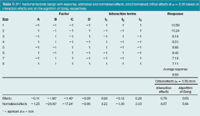
Table 1: 24–1 fractional factorial design with response, estimated and normalized effects, and (normalized) critical effects at α = 0.05 based on interaction effects and on the algorithm of Dong, respectively.

In Table 1, a 2^{4 –1} fractional factorial design is shown with the results for a given response. The effects, normalized effects, as well as the (normalized) critical effects based on interaction effects and on the algorithm of Dong are shown. It can be seen that for this response, factors B and C have a significant effect at α = 0.05. In case of method optimization, these factors could be further examined in a response surface design.⁶ When the response represents the assay results in a robustness test, then the significant factors should be more strictly controlled than was the situation in the interval examined in the design.

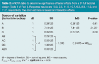
Table 2: ANOVA table to determine significance of factor effects from a 23 full factorial design (Table 1 of Part I). Response results are 10.0, 9.5, 11.0, 10.7, 9.3, 8.8, 11.9, and 11.7, respectively. The error estimate is based on interaction effects.

In some publications and software packages, the evaluation of the significance of a factor's influence on a response is evaluated from an ANOVA (ANalysis Of VAriance) approach (Table 2). For each factor, an F-test is performed. In the F-test statistic, the mean square of a factor (MS_X) is compared to that representing experimental error (MS_error),

However, the t and F-test approaches are equivalent and lead to the same conclusions when the error estimate is based on the same criterion.

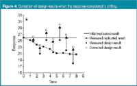
Figure 4

Occurrence of Time Effects

A special instance of the uncontrolled influences, mentioned in Section 2, are time effects in the responses. A time effect represents trends over time, which are larger than the experimental error, occurring in a response and observed at a fixed set of conditions. A drift is a special case of a time effect, which occurs when the response changes (increases or decreases) continuously in one direction over time (in Figure 4). In chromatography it can, for instance, be caused by column ageing. Such time effect will affect some estimated factor effects. In Table 3, a linear drift is affecting the response (see Drift contribution in Table 3). A given estimated effect, for example, for factor C, will reflect the effect of C plus the time effect estimated for the design column where factor C is situated. From Table 3, it is seen that mainly the estimates for factors B and C will be affected by the drift effect.

Table 3: 24–1 design with generator D = ABC and resolution IV

However, when a time effect or drift occurs, randomization of the experiments does not solve the problem of biased effects, because some estimated effects are still influenced to a certain degree by the time effect. Which are affected (most) depends on the executed sequence of the experiments.⁴ This can be observed in Table 4, where a randomized sequence of the design of Table 3 was considered. Several estimates are affected by the drift.

Table 4: Design of Table 3 in the randomized sequence 1-5-8-7-4-6-2-3

One way to minimize the time effect in the estimated effects is by using a so-called anti-drift design.^4,7 This is a screening design in which the experiments are executed in such a sequence that the main effects are not — or only minimally confounded — with the time effect, while the interactions (or dummies) are most affected. However, the estimated interaction (or dummy) effects cannot then be used in the statistical evaluation of the effects. In Table 5, an anti-drift sequence of the design of Table 3, is shown. The estimation of factor effects is minimally affected by the drift. In Table 6, a different 2^4–1 design (other generator and resolution) is shown for which an anti-drift sequence can be selected where the main effect estimates are not affected by the drift.

Table 5: Design of Table 3 in an anti-drift sequence 4-5-7-2-6-3-1

Another, and practically simpler, possibility to deal with drift effects is the execution of replicated (nominal) experiments among the design experiments (Figure 4). In this approach, when a time effect is observed, the design responses are corrected (Equation 9) relative to the (nominal) result obtained at the beginning of the experimental design to obtain proper effect estimates. The principle of the correction is shown in Figure 4. The effects estimated from these corrected responses are then as much as possible free from the time effect.

i = 1, 2, ...p and p is the number of design experiments between two consecutive replicated (nominal) experiments. y_i,corrected, y_i,measured, y_repl,begin, y_repl,before and y_repl,after are the corrected design response, the corresponding measured design response, the replicated response at the beginning of the design experiments, and the replicated responses measured before and after the design response that is being corrected, respectively.

Table 6: 24–1 design with generator D = AB and resolution III

When a drift or a time effect is observed from the replicated experiments, then effects (Equation 1) are estimated from the corrected responses. In the absence of a time effect, the measured and corrected results should lead to similar effect estimates for a given factor. In the presence of a drifting response, the normalized effects (Equation 2) are calculated relative to the result of the replicated experiment obtained before the first design experiment.

Conclusions

While in the previous column (Screening Designs, Part 1) information was supplied about screening designs and their related concepts, such as interaction effects, contrast coefficients, confounding of effects, generators, aliases, defining relation, and design resolution, in this article, concepts related to the experimental protocol and the data analysis of the design results are discussed. Moreover, the graphical and/or statistical interpretation of the estimated factor effects is overviewed.

Yvan Vander Heyden is a professor at the Vrije Universiteit Brussel, Belgium, department of analytical chemistry and pharmaceutical technology, and heads a research group on chemometrics and separation science.

Bieke Dejaegher is a postdoctoral Fellow of the Research Foundation — Flanders (FWO), working at the same department on chemometrics and experimental designs.

References

1. Y. Vander Heyden, C. Perrin, D.L. Massart, Optimization strategies for HPLC and CZE, in K. Valko (Ed.), Handbook of Analytical Separations 1, Separation Methods in Drug Synthesis and Purification, Elsevier, Amsterdam, 2000, pp. 163–212.

2. B. Dejaegher and Y. Vander Heyden, LCGC Eur., 20(10), 526–532 (2007).

3. Y. Vander Heyden et al., J. Pharm. Biomed. Anal., 24, 723–753 (2001).

4. Y. Vander Heyden et al., Robustness of Analytical Chemical Methods and Pharmaceutical Technological Products, Elsevier, Amsterdam, 1996, pp. 79–147.

5. F. Dong, Stat. Sin., 3, 209–217 (1993).

6. Y. Vander Heyden, LCGC Eur., 19(9), 469–475 (2006).

7. Y. Vander Heyden, A. Bourgeois and D.L. Massart, Anal. Chim. Acta, 347, 369–384 (1997).