Robustness Tests

Robustness testing is a part of method validation, that is performed during method optimization. It evaluates the influence of a number of method parameters (factors) on the responses prior to a transfer to another laboratory. This article describes the different steps involved to set up a robustness test and to treat its results. The approach is illustrated with a robustness test on an HPLC assay.

History, Definitions and Objectives

Because of transfer problems observed during inter-laboratory studies to assess reproducibility of quantitative methods, an intra-laboratory test indicating the problem sources was introduced.¹ It was called a ruggedness or robustness test and became a part of method validation. Initially performed at the end of the validation prior to reproducibility evaluation, it is now recommended to be executed during optimization.

It is mainly performed for assays applied in pharmaceutical analysis, mainly in industry because of the strict regulatory requirements for these methods. Different definitions have been described. The United States Pharmacopeia defines it as follows: "The ruggedness of an analytical method is the degree of reproducibility of test results obtained by the analysis of the same sample under a variety of normal test conditions, such as different laboratories, different analysts, different instruments, different lots of reagents, different elapsed assay times, different assay temperatures, different days etc."²

In fact, this definition is the same as that to estimate intermediate precision or reproducibility, for which ISO guidelines exist.³ This definition will not be discussed further. The more currently applied definition is that given by the International Conference on Harmonization (ICH): "The robustness/ruggedness of an analytical procedure is a measure of its capacity to remain unaffected by small but deliberate variations in method parameters and provides an indication of its reliability during normal usage."^4,5

An objective of a robustness test is the evaluation of factors potentially causing variability in the assay responses of the method, for example, content determinations. For this purpose, small variations in method parameters are introduced. The examined factor intervals must be representative for the variations expected when transferring the method between laboratories or instruments. The factors are then usually studied in an experimental design approach. Another objective, recommended by the ICH, is the definition of system suitability test (SST) limits for some responses, based on the robustness test results.^4,5

Set-up and Data Handling

In a robustness test, different steps can be distinguished:

• Selection of factors and their levels

• Selection of an experimental design

• Selection of responses

• Definition of the experimental protocol and execution of experiments

• Estimation of factor effects

• Graphical and/or statistical analysis of effects

• Drawing conclusions and, if necessary, taking precautions or measures.⁶

They are explained further and illustrated with a robustness test of an HPLC assay for an active compound (AC) and two related compounds (RC1 and RC2) in a drug formulation (Figure 1).

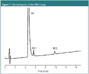
Figure 1

Selection of factors and their levels: The selected factors are related to the analytical procedure or to environmental conditions. The former are found in the method description, the latter not necessarily. Those most likely to affect the results are chosen. They include quantitative (continuous), qualitative (discrete) or mixture-related factors. For a high performance liquid chromatography (HPLC) method, some quantitative factors are mobile phase pH, column temperature, flow-rate and detection wavelength. Qualitative factors are, for instance, the batch or manufacturer of a reagent or chromatographic column. Mixture-related factors are the aqueous or organic modifier fractions in a mobile phase. For the latter factors, it is worthwhile mentioning that in a mixture of p components, only p–1 can be varied independently, which in practice means that only p–1 can be included in the designs applied for robustness testing.

Generally, two extreme levels are chosen for each factor. For quantitative and mixture-related factors, they are usually chosen symmetrically around the nominal level, described in the operating procedure. The interval should be representative for the variations, occurring when transferring the method. Extreme levels can be defined based on the experience of the analyst or estimated based on the uncertainty with which a factor level can be set and reset. They then are defined as "nominal level ± k * uncertainty" with usually 2 ≤t; k ≤ 10. The estimated uncertainty is based on the largest absolute error for setting a factor level.⁷ The parameter k is used for two reasons: (a) to include error sources not considered to estimate uncertainty and (b) to exaggerate the factor variability when transferring a method. For qualitative factors, only two discrete levels are compared.

The selected factors of the HPLC method and their levels are given in Table 1. For the quantitative, the nominal level was situated in the middle between the extremes.

In certain situations, a symmetric interval around the nominal level is not recommended. This is the case when an asymmetric interval represents more reality or when a symmetric one hides a change of response. The latter might be the case when a response is not continuously in- or decreasing as a function of factor levels. An example is, for instance, absorbance or peak area as a function of detection wavelength. Suppose the nominal wavelength is the maximum absorbance wavelength (λ_m in Figure 2). A small decrease in wavelength has a similar influence on the response as a small increase, resulting in a net effect close to zero (E_A) between both extreme levels. Here, an asymmetric interval is more informative. Only one extreme level is chosen, while the other examined is the nominal.

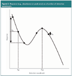
Figure 2

If the nominal wavelength (λ_n) is in a slope of the spectrum, then symmetric levels are best, since the response is continuously in- or decreasing as a function of the factor levels, resulting in the effect E_B. For qualitative factors one also preferably compares the nominal level, (e.g., nominal column), with another, (e.g., an alternative column), as shown in Table 1, (i.e., not two columns different from the nominal one were examined).

Table 1: Selected factors and their levels: low extreme, X(–1), nominal, X(0), and high extreme, X(+1), level.

Selection of an experimental design: The design selection is based on the number of examined factors and possibly on considerations related to the subsequent statistical interpretation of the factor effects. Two-level screening designs, such as fractional factorial (FF) or Plackett-Burman (PB) designs, examining f factors in minimally f + 1 experiments are used. For FF designs, the number of experiments (N) is a power of two. For PB designs, N is a multiple of four, which allows examining maximally N–1 factors. When the maximal number of possible factors is not examined, the remaining PB columns are defined as dummy or imaginary factors. For a certain number of selected factors, different possibilities exist. For example, for f = 7, FF designs with N = 8 or N = 16, or PB designs with N = 8 or N = 12, are most likely to be chosen. The eight factors from the HPLC example, for instance, are examined in a 12-experiments PB design, which is given in Table 2. A FF design with N = 16 is an alternative.

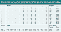
Table 2: Twelve experiments PB design to evaluate the effects of the eight factors of Table 1, (1)-(8), and three dummies, (di), on the per cent recovery, %AC, and the critical resolution, Rs(AC-RC1). The factor effects and the critical effects obtained from dummy factors, Edummies, and from the algorithm of Dong, EDong, at α = 0.05, are also given.

The screening designs allow the estimation of N–1 effects. For instance, the f = 7, N = 8 FF design results in the estimation of the seven factor effects, while that with N = 16 allows estimating 15 effects, (i.e., seven factor effects and eight so-called interaction effects). In robustness testing, the latter can be used in the statistical interpretation of effects, as will be described later in this article.

Selection of responses: Both assay and SST responses can be considered. Assay responses are, for instance, contents or concentrations of given compounds. A method is considered robust when no significant effects are found on these responses. SST responses in separation techniques are, for instance, retention times or factors of given compounds, numbers of theoretical plates, (critical) resolutions and peak asymmetry factors. Regardless whether or not the method is robust concerning its quantitative aspect, the SST responses are often significantly affected by some factors. In Table 2, two responses of the HPLC example are shown: the per cent recovery for AC and the critical resolution, Rs(AC-RC1).

Experimental protocol and execution of experiments: The sequence of experiments is then defined. Frequently, it is recommended to execute the experiments randomly to minimize uncontrolled influences on the results. However, when drift or time effects occur, for example, the change in retention time of a peak as a function of time because of the continuous ageing of HPLC columns, a random execution of the experiments does not offer a solution. A time effect is an influence on a response, making it change continuously over time because of an uncontrolled factor not examined in the design. Its influence is always confounded with a number of effects estimated from the design. As a consequence, the latter are biased and partly attributed to the drift. Which effects are most affected depends on the sequence the experiments are executed.

A first possibility to estimate drift-free effects is to execute the design experiments in a sequence that the time effect is mainly confounded with less interesting factors, for example, the dummy factors in PB designs. Such a sequence is called an anti-drift sequence. A second possibility is to correct for the drift. To do so, replicated experiments at nominal level are added to the protocol. These replicates are performed at regular time intervals before, during and after the design experiments. When a time effect is observed from the nominal experiments, all responses are corrected relative to the nominal result obtained before starting the design. This is illustrated in Figure 3. The corrected responses are then used to estimate drift-free effects.

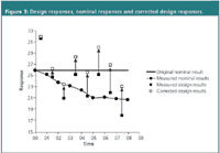
Figure 3

For practical reasons, experiments can also be blocked by one or more factors, for example, when the column manufacturer is a factor, it is more practical to first perform all experiments on one column (level), and then all on the other.

The measured solutions in each design experiment are one or more samples and standards, representative for the application of the method, i.e., taking into account concentration intervals and sample matrices. When only evaluating the robustness of a separation, a sample with a representative composition is measured. In our HPLC example, three solutions were measured: a blank, a reference solution containing the three substances, and a sample solution, representing the formulation, with given amounts of AC, RC1 and RC2.

Estimation of factor effects: The effect of factor X on response Y, E_x , is the difference of the average responses observed when factor X was at high and low level, respectively, which can be expressed as

As an example, the effects on %AC and Rs(AC-RC1) are given in Table 2.

Graphical/statistical analysis of effects: Graphically, the effects importance can be verified from a normal or a half-normal probability plot (Figure 4). In both graphs, the (absolute) effects are plotted against a value derived from a normal distribution. In these plots, points derived from a given normal distribution fall on a straight line. Here, non-significant effects, of which one expects to have most in a robustness test, fall on a straight line through zero, while the significant, which originate from another distribution, deviate from this line.

The statistical analysis usually consists of a t-test where

comparing a calculated t-value, based on the effect, E_x , and its error estimation, (SE)_e , with a critical value, based on a number of degrees of freedom depending on the (SE)_e estimation, and a significance level α. The statistic can be rewritten as

where E_critical is the critical effect. When

the effect is significant.

The error (SE)_e or the method variability can be estimated in several ways, for example, based on the variance of experiments, such as, of nominal or given design experiments, replicated under intermediate precision circumstances (not under repeatability conditions for reasons explained further). Since a robustness test is mimicking or even exaggerating reproducibility conditions, the error should be estimated under similar conditions. Thus, replicates measured at repeatability circumstances, which is often done in the literature, usually lead to an underestimation of the variability, (i.e., of (SE)_e), and to a high number of effects considered statistically significant though they are not from a practical point of view.

The error estimate can also be based on a priori declared negligible effects. In robustness testing, it concerns interaction and dummy effects for FF and PB, respectively. Another possibility is the use of a posteriori defined negligible effects, applying the so-called algorithms of Lenth and Dong. These algorithms mathematically select the effects which in the plots of Figure 4 can be considered situated on the straight line of non-significance, and use them for an error estimate. The critical effects for the HPLC example, applying the dummy effects and Dong's algorithm, are shown in Table 2.

Figure 4

Often in the literature, a statistical interpretation of effects can be found in which an ANOVA approach with F-tests is used. Such approach is in fact identical to the t-test approach.

Conclusions, precautions and measures taken: A method is considered robust when no significant effects are found for the assay responses. Otherwise, the method is not considered robust and then non-significance intervals can be defined for the significant quantitative factors. When the levels of such factors are restricted in this interval, a robust method is obtained.

As already mentioned, SST responses are often significantly affected by some factors and then SST limits can be defined, at least for situations where the assay responses are robust. SST limits can be based either on the experience of the analyst or on robustness test results, where two approaches are possible. The idea is that a given domain is evaluated by the experimental design approach, and that in this domain the assay responses are robust for all values taken by the SST responses. When defining SST limits for a given response, the experimental conditions leading to the worst result for the SST response (worst-case conditions) are selected. The SST response at worst-case conditions is then defined as SST limit, and this response is either calculated or experimentally measured.

The worst-case conditions are derived from the effects on a given response. For instance, for Rs(AC-RC1), the worst-case situation is that resulting in the lowest resolution. For the factors significantly affecting Rs, the levels resulting in the lowest Rs are selected, while for the other, the nominal is used. The corresponding Rs at these conditions is either calculated from the model,

with b₀ the average design resolution, E_i the significant effects and F_i their worst-case level, –1 or +1, or experimentally measured. For example, for Rs(AC-RC1), the calculated SST limit is 4.40, while the experimental is 4.65.

Yvan Vander Heyden is a professor at the Vrije Universiteit Brussel, Belgium, department of analytical chemistry and pharmaceutical technology, and heads a research group on chemometrics and separation science.

Bieke Dejaegher is a PhD student at the same department working on experimental designs and their application in method development and validation.

References

1. W.J. Youden, E.H. Steiner, Statistical Manual of the Association of Official Analytical Chemists, The Association of Official Analytical Chemists ed., Arlington, 1975.

2. United States Pharmacopeia, 23rd edition, National Formulary 18, Unites States Pharmacopeial Convention, Rockville, USA, 1995.

3. ISO 5725-2:1994(E), Accuracy (trueness and precision) of measurement methods and results — parts 2 and 3.

4. Validation of Analytical Procedures, Q2A Definitions and Terminology, Guidelines prepared within the International Conference on Harmonization of Technical Requirements for the Registration of Pharmaceuticals for Human Use, ICH, 1995, 1–5

5. Validation of Analytical Procedures, Q2B Methodology, Guidelines prepared within the International Conference on Harmonization of Technical Requirements for the Registration of Pharmaceuticals for Human Use, ICH, 1996, 1–8.

6. Y. Vander Heyden et al., J. Pharm. Biomed. Anal., 24, 723–753 (2001).

7. Y. Vander Heyden et al., J. Pharm. Biomed. Anal., 18, 43–56 (1998).