A Quality-by-Design Methodology for Rapid LC Method Development, Part I

This installment of Validation Viewpoint describes how statistically rigorous quality-by-design (QbD) principles can be put into practice to accelerate each phase of liquid chromatography (LC) instrument method development. Here, in Part I, the authors examine the current approaches to column screening in terms of design space coverage — a key element of process knowledge. The second part presents novel data treatments to both accelerate and bring quantitation to the column-screening effort. The third installment will focus on integrating quantitative method robustness estimation into formal method development. Moving robustness estimation upstream into the method development effort is consistent with both FDA and ICH guidances. It also enables the identification of instrument methods that simultaneously meet both mean performance and performance robustness requirements.

Michael E. Swartz

Development of analytical methods for LC instrument systems typically is carried out in two phases. The first phase involves column screening, sometimes referred to as column scouting. Column screening is the experimental work done to identify the analytical column (stationary phase) with the best selectivity in terms of all compounds in the sample that must be resolved adequately. Formal method development, the second phase, involves experimenting with additional instrument parameters believed to affect compound separation strongly. The overall goal of the two phases is identification of the instrument parameter settings that provide optimum chromatographic performance.

Ira S. Krull

This three-part column describes how statistically rigorous QbD principles can be put into practice to accelerate each phase of LC instrument method development. The column is presented in three parts. In this first part, we address column screening. We examine current method development approaches in terms of design space coverage — a key element of process knowledge. In Part II, we will present QbD data treatments to both accelerate and bring quantitation to the column-screening effort. The final installment will focus on integrating quantitative method robustness estimation into formal method development.

Traditional LC Method Development Practice

Reversed-phase LC is by far the most widely used LC separation method in the pharmaceutical and biotechnology industries. Reversed-phase LC is therefore the basis of the discussions and examples used in this paper. However, the reader will recognize that the instrumentation, software, and QbD-based methodologies presented here are applicable to other LC approaches such as normal-phase LC and hydrophilic interaction liquid chromatography (HILIC).

The traditional approach to LC method development is to systematically vary one factor across some experimental range while the level settings of all other controllable factors are held constant. This "one-factor-at-a-time" (OFAT) approach, still widely practiced today, is carried out by selecting one instrument parameter to study while holding all other parameters fixed. The "best" performing level of the study parameter is identified normally by visual inspection of the trial chromatograms; the parameter is then fixed at this level, and a new instrument parameter is selected for the next iteration. The OFAT process is repeated parameter by parameter until an adequately performing instrument method is obtained.

The OFAT approach is carried out routinely in two informal phases, with a specific set of instrument parameters relegated to each phase. The instrument parameters associated with the first phase are those that were historically "easy to adjust," meaning that new levels of the parameters could be set directly in the instrument method without the need to physically change the instrument configuration. The instrument parameters associated with the second informal phase were those for which changing a level normally required changing the instrument configuration; for example, switching a solvent reservoir or switching to a different analytical column. Table I lists the instrument parameters commonly utilized in the two informal OFAT phases of traditional method development.

Table I: Historical phasing of method development workflow

The obvious limitation of the traditional OFAT approach is that the instrument parameters that often affect selectivity most dramatically, and therefore adequate separation, are the hard-to-adjust parameters relegated to the second informal development phase. This builds inefficiency into the approach as well as risk, as critical time can be spent studying secondary affecting parameters in the first phase without achieving much performance improvement.

However, modern LC instrument systems can support column and solvent selection valves. These new automation capabilities eliminate the traditional categories of easy-to-adjust and hard-to-adjust. The experimenter is now able to select instrument parameters for study based upon relative potential to affect method performance. A direct consequence of the new automation capabilities is that LC method development protocols in many major pharmaceutical companies have promoted analytical column selection to "poll position" — that is, analytical column screening, also referred to as column scouting, now routinely constitutes the first phase of LC method development.

Figure 1 is a diagram of the LC method development workflow as it is practiced commonly today. As the diagram indicates, the first phase is analytical column selection. After the "best" column is identified, a second development phase is carried out that addresses the remaining important instrument parameters. The goal of this second phase is to identify the parameter settings that meet all critical method performance criteria, which normally include both compound separation and total assay time. After these goals are met, a separate experiment can be performed to demonstrate the robustness of the resulting method. The robustness experiment is done normally as part of the method validation effort.

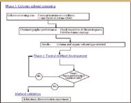
Figure 1: Current method development workflow.

This three-part series of "Validation Viewpoint" columns will apply the concept of design space in a comparison of current LC column-screening approaches. The FDA defines design space as "The multidimensional combination and interaction of input variables (for example, material attributes) and process parameters that have been demonstrated to provide assurance of quality. Working within the design space is not considered as a change. Movement out of the design space is considered to be a change and normally would initiate a regulatory postapproval change process" (1).

Screening analytical columns at fixed levels of all other instrument parameters — the OFAT approach — does not provide any process knowledge on how the candidate columns being screened would perform at other levels of instrument parameters that also can greatly affect column selectivity. To see this in terms of design space, consider pH and gradient slope — two parameters that can affect column selectivity strongly. Figure 2 illustrates a two-parameter design space delineated by typical study ranges of these parameters. Here the gradient time is held constant, and so the gradient slope is set by the final percentage of organic solvent.

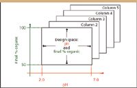
Figure 2: Design space - pH and final percentage of organic solvent.

As shown in Figure 2, the two-parameter design space must be duplicated for each column included in a column-screening study (five columns in this example), because it cannot be assumed that the parameter effects observed with one column will hold for other columns. Process knowledge of these parameters within the defined design space would be obtained by conducting an experimental design that statistically samples the design space by experimentally testing specifically defined pH–slope combinations within the space (1). However, as shown in Figure 3, the OFAT approach only evaluates each column at a single level setting combination of pH and slope, that is, screening the column at only one point within the design space. The OFAT approach therefore does not provide any process knowledge for these parameters within this design space.

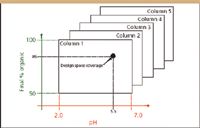
Figure 3: Design space coverage - OFAT column screening.

First-Principles Equation Approach

The most common alternative to the OFAT approach is the first-principles equation approach. This approach employs predefined equations, also called models, that predict key method-performance metrics such as retention time (t_R) of a compound as a function of one or a specific pair of LC instrument parameters within a design space. For example, a first-principles equation can predict the retention time of a compound as a function of mobile phase percent organic given reversed-phase LC, a specific column, and a specific organic solvent.

To understand how a first-principles equation relates to a design space, we must understand the structure of the equation in terms of the design space parameters. The simplest equation is the equation of a straight line relating the linear (straight-line) effect of one study variable to a response. Equation 1 is the general form of a linear equation in one variable: here y represents a response, x represents a study variable, β₁ is a coefficient that defines the slope of the line, and β₀ is the y-intercept (the value of the response, y,when the study variable, x, is set to zero). The magnitude and sign of the coefficient define the strength (steepness of the line) and direction of the variable's effect (positive or negative) on the response as it is adjusted from low to high through a defined range. The equation is therefore a model of variable behavior, because the equation can predict values of the response y for different input values of the study variable x.

Equation 2 is an example of a first-principles linear equation, which can be used to predict the retention time of a compound as a function of the percent organic solvent in the mobile phase. In this equation, k' is the retention time of the compound relative to the retention time of the void volume. S is a constant that depends upon the molecular weight of the compound, Φ is the percent of the organic solvent in the mobile phase, and k_w is the value of k' when Φ is set to zero. The equation therefore predicts values of k' for different input values of Φ.

First-principles equations for reversed-phase LC have been developed from historical experiments. Their use involves running one or two injections at different levels of instrument parameters linked to the equation. The data from these injections is used to normalize the equation, that is, improve its predictive accuracy in terms of the current sample compounds. The equation is normalized to the data using linear regression analysis, which updates the values of the equation coefficients β₁ and β₀.

Figure 4 depicts a design space in two parameters: pH and gradient time, along with two run conditions that can be used to normalize a first-principles equation such as equation 2. As shown in Figure 4, an extremely limited amount of the design space is addressed by the two normalizing runs. The first-principles equation methodology therefore operates under the assumptions that the parameter effect is represented accurately by a straight line, and that the effect is the same across the entire design space. In other words, it assumes that the effect of changing the percentage of organic solvent on the retention time is the same at any level of pH within the specified range. Another way of stating the second assumption is that the approach assumes that pH and % organic do not interact — that is, that their effects are strictly additive.

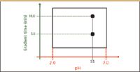
Figure 4: Design space sampling - first principles equation normalization runs.

In fact, first-principles equations that include two instrument parameters, here designated X₁ and X₂, cannot model interaction effects between the parameters. This can be seen by examining the general forms of these equations, which are presented as equations 3 and 4. Equation 3 is a linear equation in two variables; this equation can represent only linear additive effects of the variables. Equation 4 is a pure quadratic equation in two variables. The squared terms [β_ii (X_i)²] in this equation can represent simple curved variable effects (curvilinear effects). Note that neither equation contains even a simple two-way interaction term of the general form β_ij (X_i*X_j).

However, interaction effects are common among LC instrument parameters, and these effects can cause major deviations from expected behavior within a design space. In fact, the importance of interactions is implicit in the FDA definition of design space ("the multidimensional combination and interaction of input variables"). The assumption of simple additivity in the first-principles equation methodology can therefore impart significant error to the method development work. What is needed is a methodology that enables visualization and quantitation of all variable effects, which might be present in the design space.

The Classical Design of Experiments Approach

Fortunately, QbD principles can be applied to the task of screening analytical columns to include factors such as pH, gradient slope, and organic solvent type, as these factors are recognized major effectors of column selectivity. In a QbD approach, a statistical experiment design plan (design of experiments, or DOE) (1) would be used to systematically vary multiple study factors in combination through a series of experiment trials that, taken together, can comprehensively explore a multifactor design space. A statistically designed experiment can provide a data set from which interaction effects of the instrument parameters can be identified and quantified along with their linear additive effects, curvilinear effects, and even nonlinear effects.

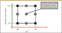
Figure 5: Design space sampling - DOE experiment.

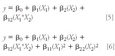
Figure 5 illustrates a DOE-based sampling plan for the two-factor design space previously discussed. The black dots correspond to a classical two-level factorial design used in initial variable screening studies. Such a design can provide data from which both linear additive effects of the instrument parameters and two-way interaction effects can be estimated from the data analysis. The two-level design enables the terms in a partial quadratic model of the form presented in equation 5 to be used in the analysis of the experiment results. The gray dots in Figure 5 correspond to the additional points that would be present in a classical three-level factorial design, also referred to as a response surface design. The addition of these points provides the data from which simple curvilinear effects also can be estimated from the data analysis. The response surface design enables all of the terms in a full quadratic model of the form presented in equation 6 to be used in the analysis of the experiment results. It is therefore considered a classical optimization experiment design.

The classical two-level design can accommodate non-numeric variables such as "Column Type" in which the two levels correspond to two different columns. However, the classical three-level designs, which support the full quadratic equation, require numeric variables, and so cannot be used for screening more than two columns at a time. Fortunately, there is another type of DOE design, referred to as an algorithm design, that can construct and statistically sample more complex design spaces such as those that include multiple levels of both numeric and categorical variables. These advanced DOE designs also support more complex analysis model forms that can estimate interactions between categorical and numeric variables as well as nonlinear variable effects.

As previously mentioned, the new automation capabilities of most modern LC instrument systems have eliminated the traditional categories of easy-to-adjust and hard-to-adjust. Coupling advanced DOE designs with automation enables the new phased method development approach to include multiple analytical columns in combination with critical parameters such as pH and organic solvent type — parameters known or expected to have column-dependent effects. The second phase of method development then includes remaining instrument factors that also can affect separation. These factors are studied to further optimize method performance. Table II lists the instrument parameters commonly utilized in the new approach to phased method development.

Table II: Current phasing of method development workflow

In practice, column-screening experiments, even those done using a design of experiments (DOE) approach, often have significant inherent data loss in critical results such as compound resolution. The data loss is due to both compound co-elution and also changes in compound elution order between experiment trials (peak exchange). These changes are due to the major effects that variables such as pH and organic solvent type can have on the selectivity of the various columns being screened. Switching columns between trials while simultaneously adjusting these factors dramatically affects compound elution and therefore the completeness of the resolution data obtained from the experiment trial chromatograms.

Part II of this series will describe the data loss inherent in most column-screening experiments due to co-elution, peak exchange, and the general difficulty of accurately identifying peaks across the experiment trial chromatograms (peak tracking). Such data loss will be seen to make numerical analysis of the results very problematic. It often reduces data analysis to a manual exercise of viewing the experiment chromatograms and picking the one that looks the best in terms of overall chromatographic quality — a "pick-the-winner" strategy. Part II will then describe Trend Responses, a novel type of results that can be derived directly from experiment chromatograms without peak tracking. Trend responses overcome the data loss inherent in traditional column-screening studies, and so enable accurate quantitative analysis of the experiment results.

Conclusions

Chromatographic analytical method development work normally begins with selection of the analytical column, the pH, and the organic solvent type. A major risk of using either an OFAT approach or a first-principles equation approach in this phase is that these approaches provide extremely limited coverage of the design space. This limitation translates into little or no ability to visualize or understand the interaction effects usually present among these key instrument parameters.

Alternatively, a QbD-based methodology employs a statistically designed experiment to address the design space comprehensively and enable the experimenter to visualize and quantify all important variable effects. However, this approach often results in significant inherent data loss in key chromatographic performance indicators such as compound resolution due to the large amount of peak exchange and compound coelution common in these experiments. Inherent loss makes it difficult or impossible to quantitatively analyze and model these data sets, reducing the analysis to a pick-the-winner strategy done by visual inspection of the chromatograms.

Acknowledgments

The authors are grateful to the Elanco Animal Health Division of Eli Lilly and Company, Inc., and to David Green, Bucher and Christian, Inc., for providing hardware, software, and expertise in support of the live experimental work presented in this paper. The authors also want to thank Dr. Graham Shelver, Varian, Inc., Dr. Raymond Lau, Wyeth Consumer Healthcare, and Dr. Gary Guo and Mr. Robert Munger, Amgen, Inc. for the experimental work done in their labs that supported refinement of the phase 1 and phase 2 rapid development experiment templates.

Joseph Turpin is an Associate Senior Scientist with Eli Lilly and Company, Inc., Greenfield, IN. Patrick H. Lukulay, Ph.D. is the Director, Drug Quality and Information U.S. Pharmacopeia Rockville, MD.

Richard Verseput is President, S-Matrix Corporation Eureka, CA.

Michael E. Swartz "Validation Viewpoint" Co-Editor Michael E. Swartz is Research Director at Synomics Pharmaceutical Services, Wareham, Massachusetts, and a member of LCGC's editorial advisory board.

Ira S. Krull "Validation Viewpoint" Co-Editor Ira S. Krull is an Associate Professor of chemistry at Northeastern University, Boston, Massachusetts, and a member of LCGC's editorial advisory board.

The columnists regret that time constraints prevent them from responding to individual reader queries. However, readers are welcome to submit specific questions and problems, which the columnists may address in future columns. Direct correspondence about this column to "Validation Viewpoint," LCGC, Woodbridge Corporate Plaza, 485 Route 1 South, Building F, First Floor, Iselin, NJ 08830, e-mail lcgcedit@lcgcmag.com.

References

(1) ICH Q8 - Guidance for Industry, Pharmaceutical Development, May 2006.

(2) L.R. Snyder, J.J. Kirkland, and J.L. Glajch, Practical HPLC Method Development, 2nd ed. (John Wiley and Sons, New York, 1997).

(3) J.A. Cornell, Experiments With Mixtures, 2nd ed. (John Wiley and Sons, New York, 1990).

(4) M.W. Dong, Modern HPLC for Practicing Scientists (John Wiley and Sons, Hoboken, New Jersey, 2006).

(5) D.C. Montgomery, Design and Analysis of Experiments, 6th ed. (John Wiley and Sons, New York, 2005).

(6) R.H. Myers and D.C. Montgomery, Response Surface Methodology (John Wiley and Sons, New York, 1995).