How Many Repetitions Do I Need? Caught Between Sound Statistics and Chromatographic Practice

In chromatographic analysis, the number of repeated measurements is often limited due to time, cost, and sample availability constraints. It is therefore not uncommon for chromatographers to do a single measurement. If measurements are repeated, it tends to be duplicates or triplicates. However, statistical principles dictate that a sufficient number of replicate measurements are necessary to ensure reliable and robust data interpretation. This article examines the required number of repetitions from a statistical perspective.

No peak integration is flawless, as the previous instalment of “Data Analysis Solutions” highlighted (1). To learn how to process our data, it is thus paramount to understand what contributes to the quality of data. Fortunately, the lack of perfection is nothing new to our chromatographic community. We have long accepted that, no matter how hard we try, no pump, column, detector, or analyst will ever be perfect.

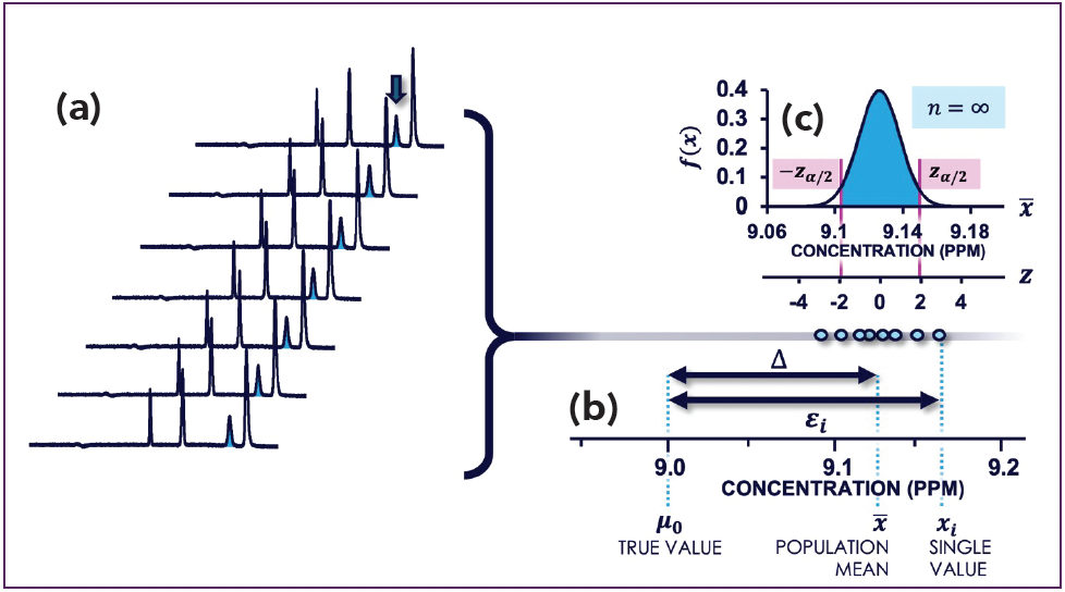
Indeed, any measurement (x_i) we take of our variable of interest (x) contains some error (ε_i). Figure 1a shows an example of seven chromatograms where the peak belonging to the reference standard is marked with an arrow. In Figure 1b, we see that the error causes a data point x_i to be different from the actual true value (µ₀). If we would take a large number of repeated measurements, we can say that the total error can be split (decomposed) into two components contributing to it:

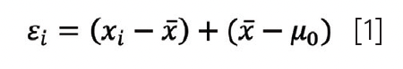
where x̄ depicts the mean of the replicates. In equation 1, (x̄ – µ₀) represents the systematic error, or bias, Δ, of our measurements. It can be determined using reference materials, certified standards, or interlaboratory trials. From the perspective of data analysis, there is little we can do about systematic errors except to be aware of them and—where possible—correct appropriately. We will thus continue this article under the assumption that such errors are absent.

Figure 1: (a) Sample of seven chromatograms from which there is one peak of interest; (b) Key definitions of errors in quantitative analysis for the sample seven data points; (c) Normal distribution representing the full population of an infinite number of replicates that could have been taken of the analyte mixture. Adapted and reproduced from (2), with permission from the Royal Society of Chemistry.

However, (x_i – x̄) represents the random error that results in a spread of the measurements around the sample mean. It can also be expressed using a descriptive statistic as the precision, or standard deviation, s, of our method.

Wait, s? Shouldn’t this be σ? Well, no. In statistics, we use the Greek alphabet (µ and σ) to denote statistics that describe the population of the infinite number of replicate measurements we theoretically could do. Figure 1c shows how the random measurement error for this case is expressed with a normal distribution that is described by µ and σ. This distribution is also referred as a probability density function (PDF), as it describes the probability of finding a value. There is always a 100% chance of finding a value and the PDF therefore has the convenient property that the area under the curve is equal to 1.

In quantitative analysis, we take a sample (that is, a limited number) of measurements to describe the population. The Latin alphabet (x̄ and s) is used to denote statistics that describe such a sample. In other words, we use x̄ based on our measurements to say something about µ.

Confidence Intervals

The problem now becomes that, given that the individual measurements vary, it is also unlikely that—even in the absence of systematic errors—the mean of our sample x̄ is exactly equal to the true value µ₀. If our repeated measurements cannot provide a reliable answer on the samples submitted for analysis, then what can?

It is precisely for this reason that we typically calculate a range of values that is likely to include the true mean (µ₀). We refer to this range as the confidence interval. This range depends on the significance level (α) and expresses how confident we are with our estimation of µ. We will discuss the meaning and implications of in a future installment. For now, it is sufficient to understand that α is 0.05 for a 95% confidence interval, and 0.01 for a 99% confidence interval. The confidence interval can be computed using:

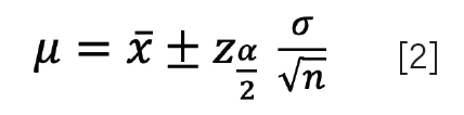
Here, x_α/2 is the critical value, also denoted as Z_crit, which is obtained by converting the data using the standard distribution (Z = (x – µ)/σ). Here, Z follows a normal distribution with a µ of 0, and a σ of 1. Conveniently, Z_crit is always 1.96 for a 95% confidence interval (we often say that 95% of our data lies between ±2σ of the mean, but it is actually ±1.96σ).

One disadvantage of equation 2 is that it requires σ to be known. Unfortunately, we do not have an infinite number of measurements of the population, only our limited sample of n measurements, and thus our measure of the variation of x is represented by i. While s can be a measure of σ, we will see below that this only holds for a sufficiently large number of repeated measurements (n > 30). This is not a very realistic number in practice.

Degrees of Freedom

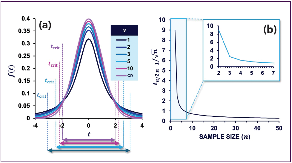
Arguably, chromatographers usually speak of a duplicate or triplicate when we do replicate measurements. However, as we decrease the number of replicates, we can expect to become less confident about our determination of µ. This is captured by the Student’s t-distribution, which owes its name to William Sealy Gosset who introduced it under the pseudonym “Student.” Unlike the normal distribution, the t-distribution is not described by µ and σ, but by the degrees of freedom, ν, which is equal to the number of measurements minus one (ν = n – 1). Figure 2a shows a plot of the PDF of the t-distribution for different values of ν. The t-distribution becomes much wider as decreases, thus reflecting the increasing uncertainty. This is also reflected by the critical values (t_crit) for the 95% confidence interval, which are 12.71 (ν = 1), 4.3 (ν = 2), 3.18 (ν = 3), 2.57 (ν = 5), 2.23 (ν = 10), and 1.96 for (ν = ∞). Indeed, at ν = ∞, the t-distribution becomes identical to the normal distribution.

Figure 2: (a) t-distribution plotted for different degrees of freedom. The
distribution widens dramatically at low values of replicates; (b) The component
t_(α/2),v/√n of equation 3 plotted against n shows that a sevenfold improvement
in the confidence interval may be obtained when five repeated measurements are taken instead of just two. Adapted and reproduced from (2), with permission from the Royal Society of Chemistry.

The confidence interval of the mean for small samples can now be defined as:

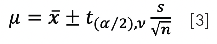
where t_(α/2),v, or t_crit, is the critical value at significance α with degrees of freedom ν. Figure 2a shows that the range that is likely to contain the true mean is becoming wider. A grim realization is that the practical triplicate (ν = 2) and duplicate (ν = 1) are not even depicted in Figure 2a.

So, what number of replicates is sensible? We see that equation 3 comprises of several components: (i) the precision, (ii) critical t-value (t_crit) and (iii) √n. In Figure 2b, the combination of the components t_crit and √n are plotted as a
function of n. The curve shows a dramatic narrowing of the confidence interval for the first 10 replicates, with the improvement significantly diminishing at higher numbers. It is for this reason that above n > 30, statisticians usually consider s a reasonable estimate of σ. In any case, the inset of Figure 2b shows that a duplicate may not be very meaningful (albeit better than a single measurement) and that having five instead of two replicates leads to a sevenfold narrowing of the confidence interval: the first five experiments definitely pay off.

Readers interested in applying these concepts can click here.

References

(1) Pirok, B. W. J. Resolving Separation Issues with Computational Methods, Part 2: Why is Peak Integration Still an Issue? LCGC Intern. 2024, 1 (6), 20–21. DOI: 10.56530/lcgc.int.ja6279m5

(2) Pirok, B. W. J.; Schoenmakers, P. J. Analytical Separation Science; Royal Society of Chemistry, 2025.

About the Author

Bob W. J. Pirok is an associate professor of analytical chemistry at the Van ‘t Hoff Institute for Molecular Science (HIMS) at the University of Amsterdam. He is the author of the educational textbook Analytical Separation Science, which is set to released in May 2025. Direct correspondence to B.W.J.Pirok@uva.nl