Effects of External Influences on GC Results

John V. Hinshaw, GC Connections Editor

Small differences in process gas chromatography (GC) results from the same sample stream over time can indicate corresponding changes in target analyte concentrations, or the fluctuations might be due to external influences on the instrument. This instalment of ”GC Connections” explores ways to examine such results and better understand their significance.

I sometimes become involved in conversations that start out with casual observations about data variability and the closeness or lack thereof between two or more sets of analytical results originating from the same material source. Sometimes differences may be expected, especially when, for example, two very different methodologies are compared. In other cases, a lack of closeness between sets of results could indicate a problem that needs attention. This instalment of “GC Connections” explores some of the basics and then examines some real‑world data to see what can be learned or at least inferred. 

The Problem of External Influences 

A collection of experimental data with multiple external influences comes with a problem: Is the apparent meaning of the observations influenced by unaccounted experimental factors? In chromatography, as in other experimental methods, we try to control as many external factors as possible. For example, a tank pressure regulator may be susceptible to the gas flow rate through it, causing its outlet pressure to change significantly as flow changes. The inlet pressure and flow controllers in a gas chromatography (GC) instrument are designed to compensate for this variability. However, if the tank regulator is not configured correctly with an outlet pressure at least 10% higher than the highest column inlet pressure, the ability of the GC system pneumatics to perform accurately may be compromised. This inaccuracy in turn can lead to irreproducible retention times and thus result in poor performance.

A list of some possible external influences includes:

• environmental temperature and pressure,

• main power line voltage and frequency,

• carrier and detector gas purity,

• condition of gas generators,

• service state of in-line gas filters,

• condition of pressure regulators, and

• leaks in connecting tubing.

• Factors internal to a GC system that can influence chromatographic results also include:

• inlet liner type and condition,

• state of the detector, such as flame jet cleanliness,

• internal gas leaks or blockages,

• column inlet and outlet connections,

• column contamination and age, and

• inlet, oven, and detector temperature control.

Chromatographic and other experimental results benefit tremendously by users understanding and controlling as many of these factors as possible. The influences listed above are not intended to be comprehensive lists, but rather points of discussion. Considerations for the influence of sampling and sample preparation as sources of error are beyond this discussion, and I am sure readers can name even more factors to worry about. 

A real problem arises when such influences are either not identified or cannot be compensated for. Let’s review some data with an external influence that can be readily identified and understood.

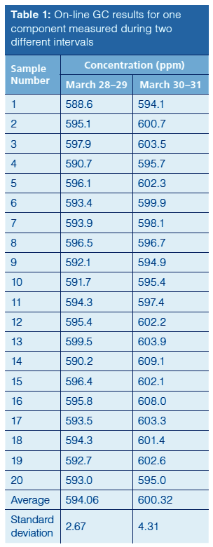
Table 1 gives measured concentrations and simple statistics for a single component measured by a process GC system during two contiguous intervals of two days each. Visual inspection appears to confirm that the two data sets measure different concentrations. The arithmetic means differ by about the same amount as the standard deviation of the second set of data, and by about twice the standard deviation of the first set of data. But how significant are the differences? Can the conclusion be drawn that the concentration being measured has changed from one set of data to the next?

Most readers will be familiar with Student’s t-test. An interesting point of fact: the attribution to Student refers to the pseudonym used by Willam S. Gosset who in 1908 published the test as a way to monitor the quality of stout beer at Guinness in Dublin, Ireland.

The t-test infers information about a larger population from relatively few samples. It is based on the assumption that the population being sampled falls close to a normal or Gaussian distribution of values. The t-distribution is a probability density function of the number of degrees of freedom (df) in a sample set. For a single set of n measurements, df = n – 1. As degrees of freedom increase beyond about 60, the t-distribution approaches a normal distribution. At lower levels, it predicts the entire population’s characteristics on the basis of the fewer available samples. As we shall see, and much like chromatographic peaks, this assumption can be incorrect for real‑world data. 

The t-test is most often applied to a single set of data in comparison to a single known value, to determine the significance of the hypothesis that the data represents the same value as the known amount. The t-test can also be applied to two data sets in comparison to each other, but it assumes that the variances of the sampled populations are the same, and it works best if the number of samples or degrees of freedom of each sample set are the same as well. This last assumption is true for the data in Table 1, but the variances, which are the squares of the standard deviations, are obviously not the same. This difference is an indication that some unaccounted influence may be at work inside the data.

There are several alternatives to the basic t-test. In the present case, Welch’s unequal variances t-test seems the most appropriate. This modification accommodates unequal population variances, although it still assumes that the population variances are normal. Performing Welch’s t-test gives a null‑hypothesis probability (p-value) of ~2 × 10-6 that the mean values are not different or, to put it another way, the probability that the sample means are different seems to be greater than 99.999%.

The data analysis might stop at this point, and we might conclude that the quantity being measured has changed from the first sampled interval to the second. However, the significantly different variances or standard deviations of the two sample sets should lead to further investigation.

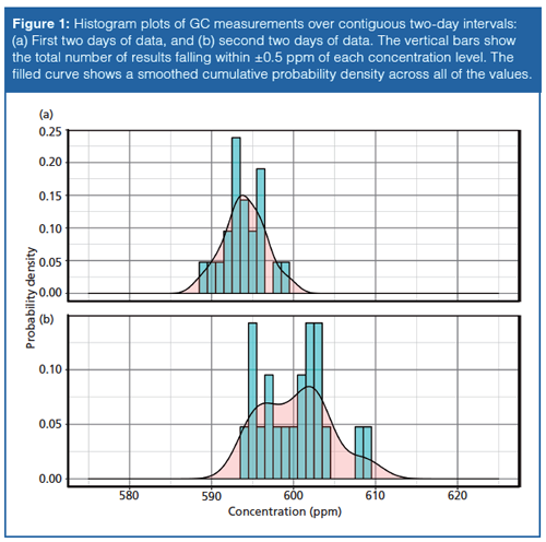
The two sample data sets are plotted in Figure 1 as histograms, where the height of each bar represents the number of samples with values between regular intervals along the x-axis. In this case, the intervals are spaced at 1-ppm increments. For the first set of data, there are two values at 595 ± 0.5 ppm at the points 595.3 and 595.4, while for the second set there are three values in the same interval, at 594.9, 595.0, and 595.4. The smooth filled curve in each plot shows a calculated probability density that a sample falls at a particular concentration, and helps visualize the distribution of the measured values. The values have a normal-looking distribution for the first sample set but definitely not for the second one.

Another useful visualization is a time-series plot of the data. This plot can help you see if there is some systematic factor that varies over time and has an influence on the measurements. Figure 2 is a time-series plot, with the measurement data in the upper panel and the bulk sample-stream temperature in the lower panel. There is a clear correlation between sample temperature and measured concentrations. The peak-to-peak sample temperature fluctuates a bit more in the second sample set than in the first, which could explain the larger observed standard deviation in the second set. The peaks and valleys of the concentration measurements tend to lag behind the sample temperatures by some hours. This time lag is an expected behaviour in the process system under test because of the flows and volumes involved, although there is no room here to provide more detail. A clear upward trend in sample concentration is also apparent in the second set of observations, while the sample temperature moves about a relatively constant value.

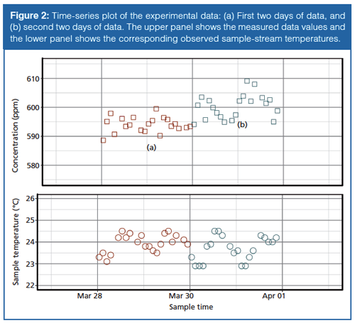
The upward trend makes simple t-test results less meaningful. We no longer have an unchanging population to sample; it has changed while we observe it. This fluidity strongly contributes to the apparent variance of the test data. How to proceed with data analysis depends on the measurement goal. Do we want to know whether the concentration changes over a shorter or longer time span? Smoothing or removing the thermal influence from the data could remove much of the periodic nature of the results and reveal a more clear picture of how the results increase over longer time spans, while making measurements more frequently would improve the short-term characterization. There may be, and probably are, other external influences on the results. As a whole, the external factors tend to couple together, as well, which correlation techniques such as principal component analysis can help unravel.

Conclusion

This brief data analysis shows the influence of temperature on measured results. Although the system under test was not a typical laboratory setup, it demonstrates how a simple statistical analysis of measured results can provide misleading information about the variability of the results and the influence of external sources. It also shows that analysts can better understand how their systems are affected by outside influences, and then proceed to take control of the variables they can while accommodating those they cannot change.

“GC Connections” editor John V. Hinshaw is a Senior Scientist at Serveron Corporation in Beaverton, Oregon, USA, and a member of LCGC Europe’s editorial advisory board. Direct correspondence about this column to the author via e-mail: lcgcedit@lcgcmag.com