Detangling the Complex Web of GC×GC Method Development to Support New Users

The introduction of comprehensive two-dimensional gas chromatography (GC×GC) to the sample screening toolbox has substantially increased the ability to comprehensively characterize complex mixtures. However, for many gas chromatography (GC) users, the thought of having to learn to develop methods on a new technology is daunting. Developing a basic GC×GC method for most (nonspecialized) applications can be accomplished in minimal time and effort given parameter suggestions and ranges to target analytes in a sample of interest. In this article, we work through a simple workflow to develop a GC×GC method for a specific sample upon initial use, with the aim of decreasing the time to accomplish functional workflows for new users.

Gas chromatography (GC) is generally regarded as the gold standard for analyzing mixtures of volatile and semi-volatile components. More recently, comprehensive two-dimensional gas chromatography (GC×GC) is becoming increasingly popular for the screening and exhaustive analysis of complex samples in scenarios where one-dimensional GC (1D-GC) peak capacity is limited (1). This separation technique utilizes two columns connected via a modulator to separate components of a mixture. The columns must each have a different stationary phase coating, allowing independent retention mechanisms on each column and increasing peak capacity for complex separations in the gas phase. GC×GC is often coupled with time-of-flight mass spectrometry (TOF-MS) due to the need for fast mass spectral acquisition that can limit mass spectral skewing and generate quantitative data.

GC×GC has often been viewed as a technique that should remain in the research space and may never become common practice for routine analysis environments. Nevertheless, the industrial and commercial user base of GC×GC continues to increase in size and grow into new applications, providing promise of its graduation to a fully mature technique within the chromatography toolbox. While the complex interplay of different GC×GC parameters has been well characterized in prior GC×GC research (e.g. the historical “spaghetti diagram”) (3,4), an increase in commercial options and reliable recommendations from instrument manufacturers has substantially decreased the complexity and activation barrier to implementing a thoughtful GC×GC method when getting started with this technique. In this guide, we begin with the use of an open-source modeling tool to optimize the first dimension separation, inject samples first using a 1D-GC method and a respective GC×GC method based on general recommendations, and suggest a series of possible initial method development experiments. This workflow can be achieved in one or two days and results in an acceptable GC×GC method for further testing. The intention of this work is to present the basic steps in developing a valuable GC×GC method to new users to demystify the method development process in moving towards GC×GC technology.

The workflow presented required the use of a complex sample. As such, a 48-component Indoor Air Standard (Millipore Sigma, St. Louis, MO, USA) was used as a sample of interest. It is also possible to use the same workflow on any real sample that is not a chemical standard. The standard was obtained in a stock solution of 1000 ppm and was diluted with high-performance liquid chromatography (HPLC)-grade methanol (Fisher Chemical, Fair Lawn, NJ, USA) to a nominal concentration of 5 ppm in a 2 mL GC vial. HPLC-grade methanol was also used for blank injections before and after each sequence, as well as in between every 10-15 samples for longer runs. Samples were analyzed using a Pegasus BT4D GC×GC–TOF-MS equipped with an LPAL3 autosampler and a quad-jet dual stage cryogenic modulator (LECO Corporation, St. Joseph, MI, USA).

First, the desired analytes were entered into the Restek Pro EZGC Chromatogram Modeler (5). In a scenario where desired analytes are not actually known, a sample can be run in 1D GC mode to identify analytes of interest on any literature method as a starting point. This modeler allowed the adjustment of basic parameters like column choice, oven ramp rate, and pressure settings to generate a desirable 1D-GC separation. For the compounds of interest in the air standard, results could be viewed in 1D across a nonpolar, polar, or mid-polar column choice. Although it was not possible to select the exact column used within our instrument, knowledge of the most similar stationary phase to the column in our system supported choice of the best result.

Following the initial exploration on the chromatogram modeler software, a base method was constructed to serve as a starting point for the run. The method was first created in GC×GC mode, and then a second method was created by saving over this initial method and disabling the GC×GC options to allow a 1D GC run for comparison. This disables the modulator but keeps the modulator and secondary oven temperatures on to provide the most realistic comparison of 1D and GC×GC methods, while preventing physical column changes. Desired analytes were identified in ChromaTOF v. 5.56.53 (LECO Corporation) in both 1D and GC×GC mode. For the current study, starting parameters are listed in Table 1. Note that for this study, the popular default combination of a non-polar 5% diphenyl/dimethylpolysiloxane first dimension column and semi-polar 17% diphenyl/dimethylpolysiloxane second dimension column was used. The specific column combination was an Rxi-5ms in the first dimension and an Rxi-17Sil MS in the second dimension (Restek Corporation).This conforms with popular methods in literature, but also allows use of higher temperatures in heated zones, enables comparison against traditional retention index values for component identification, and provides the benefit of ordered chromatograms based on analyte structure (6). Afterwards, problematic areas of the chromatogram were identified (i.e. locations where baseline separation and peak shape were not desirable). Finally, further development was conducted on the sample of interest within the GC×GC method.

Six parameters were part of the optimization process as shown in Table 2: modulation period, oven hold time at the start of the run, oven hold time at the end of the run, oven ramp rate, hot pulse time, and secondary oven offset temperatures. The first four of these parameters were tested together with three options for each parameter. Once a modulation period was decided upon, hot pulse times and secondary oven offset temperatures could then be optimized using the decided upon modulation period. Cold pulse time was always represented as the remaining time after hot pulse time was set.

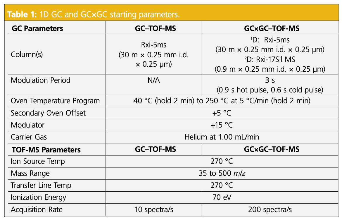
Using the open-source chromatogram modeler, different column parameters were analyzed for elution efficiency. Knowing the 48 components that were in the Indoor Air Standard, it was helpful to use this chromatogram modeler to envision how many components would elute and to identify any problematic regions of congestion in the chromatogram. Some features of the modeler include “not found” compounds, “refine oven program,” and the possibility to change columns with the click of a button. The software also provides measured resolution values for each peak and highlights when peak resolution is below the target set by the user. In addition to changing stationary phases, there are some options to change column length, internal diameter, and film thickness. The “not found” compounds are ones that were not shown in the chromatogram, so having this knowledge allowed parameters to be changed to improve chromatographic resolution. The modeler option “refine oven program” was used to increase the number of compounds separated, and flow rate of the carrier gas was also adjusted to improve separation. These options can help to provide a high quality first dimension separation drastically before even considering the secondary column applied in GC×GC. The closest column polarity compared to the 5% diphenyl/dimethylpolysiloxane on the modeler was 1% diphenyl/dimethylpolysiloxane and the results of this selected column are shown below in Figure 1 (top) alongside the results of the initial 1D-GC run on the instrument (bottom).

The 1D chromatograms produced from the indoor air standard contained multiple instances of co-elution. Often, areas that looked like only one or two peaks in 1D-GC could be further resolved and visualized better using GC×GC. For this reason, the improved visibility of GC×GC was desirable. Note that in this sample, all analytes were at comparable concentrations without any other matrix interferences. However, a real air sample would likely contain a broader dynamic range and other introduced compounds, and therefore, the chromatographic situation can be much more complex than presented in Figure 1. The most challenging areas of the 1D-GC run for resolution proved to be the first few minutes of the run and a region around 10 min, which was confirmed when running the method on the sample.

Moving to optimizing the GC×GC parameters, the first set of experiments was run as a single sequence to optimize modulation period, primary oven hold time at the beginning of the run, primary oven hold time at the end of the run, and primary oven ramp rate. The results of the modulation tests are shown first in Figure 2. This is a great parameter to start with, as you can typically choose a short, long, and mid-range modulation period to get a sense for the maximum retention in the second-dimension column, then cut your modulation period to the most appropriate point. In Figure 2, it was apparent from the comparison of the three modulation periods that the compounds exhibiting the most retention in the secondary column did not elute past 1.2 s. Therefore, the modulation period was chosen as 2 s, to use optimal space on the GC×GC plot.

It is also important to note that while the compounds look “wider” in the second dimension in the top plot, they are not actually wider than the middle or bottom plots, but rather represent more of the modulation period y-axis scale. This comparison is also a good way to monitor for possible analytes that may be prone to wraparound. This phenomenon can sometimes be a problem due to band broadening of a peak while being retained in the second-dimension column beyond the modulation period in which it enters.

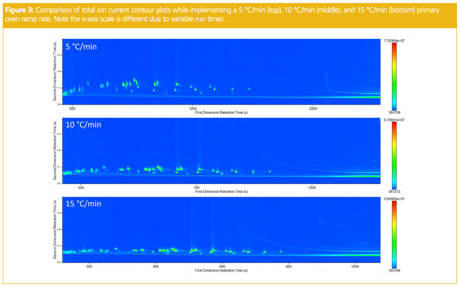
Although in 1D-GC it can sometimes be common to implement stepwise increases or holds within the oven ramp to target areas of co-elution that are problematic, it prevents the ability to use traditional linear retention indices to assist in compound identification. A slower ramp rate will allow the compounds additional time to resolve, while a faster ramp rate will move analytes through the column with less interaction. The results of the ramp rate comparison are presented below in Figure 3, with 5 °C/min being selected as the most ideal ramp for this sample. This test helped to confirm that the run time would be sufficient in resolving compounds from one another in the first dimension. Finally, the start and end oven hold times were also compared. Increasing the hold times longer than 2 min at the start and end of the run did not result in any improved results and thus 2 min was selected at the start and end of the run.

After determining modulation period (2 s), primary oven ramp rate (5 °C/min), initial oven hold (2 min) and final oven hold (2 min), these parameters were input into the method and two final parameters were tested, which included hot pulse time and secondary oven offset. The hot and cold pulse times are linked, and it is generally recommended to select a hot pulse time that is 30% of the modulation period. Thus, with a modulation period of 2 s, the hot pulse time should be ideal at 0.6 s, resulting in a cold pulse time of 0.4 s. The hot and cold pulse time will add to half of the modulation period, since the modulator used in this study is a dual-stage modulator. Although we tested three different hot and cold pulse configurations, no major differences were observed and thus the 30% recommendation was selected.

Finally, the secondary oven offset can be used to control movement through the secondary column during the modulation period. The general recommendation is to operate the secondary oven at a +5 °C offset to the primary oven, to keep compounds moving efficiently through the column. However, it can also be increased to a higher value if, for example, there is minor wraparound of analytes in the second dimension and a longer modulation period cannot be applied. The results of the secondary oven offset experiment are shown in Figure 4 for a subset of the chromatogram. Although the difference in space along the y-axis may seem subtle at first glance, the two analytes at 650 s have much better second dimension resolution, as well as the three peaks appearing before 750 s.

While the peaks are resolved in all three method options, if additional interferences were present in this sample, this increased second dimension resolution may be helpful. It would also be important if one of the two compounds were saturating while the other was trace in amount. These types of assertions can often be made when looking at a real sample for method development whereas the use of standards does not always convey this complexity.

It is also possible to perform additional optimization on the modulator offset, which for our system is recommended to be +15 °C compared to the secondary oven temperature. However, as the secondary oven offset was already selected, the default recommendation was taken. In general, if the modulator offset exceeds the primary and secondary oven temperatures, this should provide enough temperature to keep compounds moving forward efficiently through the modulator.

Conclusions

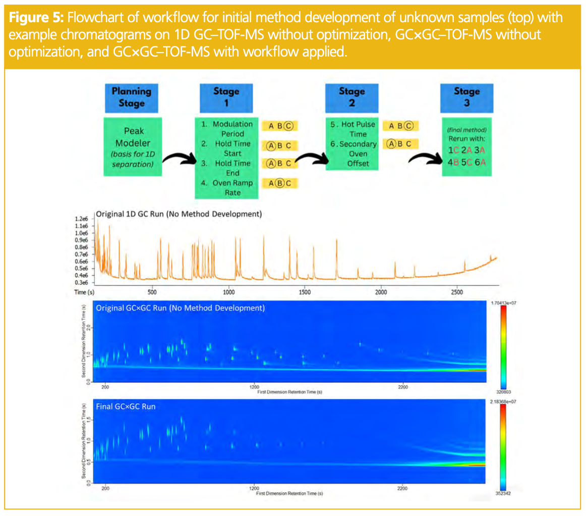
When dealing with a new method implementation that involves several parameters, it can be intimidating to consider how these parameters interplay, which setting to tackle optimizing first, and how to make informed decisions to obtain the best results. However, through using a simple workflow shown in Figure 5, it is possible to work through these steps mindfully and at the very least, determine when small method adjustments do not yield major chromatographic improvements. New users to GC×GC, especially in routine analysis environments, are often interested in a simple workflow to get started, and the workflow presented herein is a good approach to development. Additional statistical optimization may yield small improvements to the method, but following this workflow should result in a usable method that fits the desired purpose. Figure 5 displays the general workflow described and the result of the sample run with all parameters finalized.

Another important consideration often ignored in the research laboratory is method similarity between different applications. Extremely complex and lengthy optimization protocols that produce incremental or marginal improvements often result in methods that are highly fit for a specific purpose but rarely translate well across several applications. For laboratories running different types of samples, having a general method may be more important for cost and sample throughput than having a highly unique method for each type of work. In this way, method development is often a balancing act that comes with compromises. There is no single “right” method for a sample of interest. However, taking basic steps to test method parameter options can assist new users in developing a method that is ready to implement within a short time and with relatively little need for extensive training or consultation with experts.

The authors would like to thank the Restek Academic Support Program for support with project consumables. LECO Corporation is also acknowledged for support with the instrument and optimization workflow. Additionally, the authors acknowledge the William & Mary Chemistry Department for support with supplies and technical support from Jeff Molloy, Director
of Laboratories and Instrumentation.

The PI is also funded through the Henry Dreyfus Teacher Scholar Award by the Camille & Henry Dreyfus Foundation.

References

(1) Zanella, D.; Focant, J.; Franchina, F. A. Analytical Science Advances 2021, 2 (3–4), 213–224.

(2) Harynuk, J.; Gorecki, T. Am. Lab. 2007, 39 (4), 36–39.

(3) Mostafa, A.; Edwards, M.; Górecki, T. Optimization Aspects of Comprehensive Two-Dimensional Gas Chromatography. J. Chromatogr. A 2012, 1255, 38–55.

(4) Restek Corporation. Restek ProEZGC Chromatogram Modeler. https://ez.restek.com/proezgc (accessed June 3, 2023).

(5) Stefanuto, P.-H.; Focant, J.-F. Columns and Column Configurations. In Basic Multidimensional Gas Chromatography; Snow, N., Ed.; Academic Press, 2020; pp. 69–88.

E-mail: kaperrault@wm.edu.com

Website: www.wm.edu