Count the Cost, Part II: Increasing Resolution by Increasing Retention
LCGC North America
We’ll see how to find the “sweet spot” in terms of retention for a liquid chromatographic separation as well as how much retention change is to be expected for a selected change in mobile-phase percent organic or column temperature.
We’ll learn how to find the “sweet spot” in terms of retention for a liquid chromatography separation as well as how much retention change can be expected for a selected change in mobile-phase percent organic or column temperature.
This is the second installment in a series about how to use chromatography fundamentals to estimate the impact of various parameter changes on liquid chromatography (LC) separations. In the first discussion (1) we looked at the influence of the column plate number (N) and saw that for most situations, starting method development with a 10,000-plate column makes the most sense. This is a good compromise between separation power, pressure, and run time. The effect of further changes in column length (L) or particle diameter (dp) can be easily estimated without doing the actual experiments.
This month, we’ll continue the discussion with an emphasis on the influence of the retention factor (k) on the separation, expressed as resolution (Rs). We’ll consider the general case, specific cases, and how to estimate the influence of a change in mobile-phase percent organic (%B) or temperature on retention. As with the prior installment of this series, we’ll limit ourselves to isocratic separations and reversed-phase conditions to simplify the discussion, but much of this installment will apply to gradients and other separation modes.
The Influence of Retention on Resolution
Once again, we’ll use the fundamental resolution equation to guide the discussion:

where α is the selectivity between two peaks with k-values of k1 and k2:

Although we could use retention time (tR), it is usually simpler to use the retention factor in discussions like the present one. Recall that the retention factor is calculated from tR and from the column dead time (t0 or tM) as:

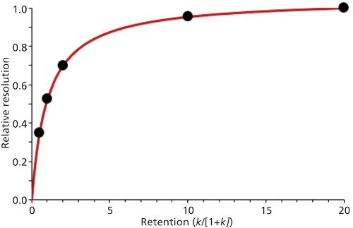
From equation 1, we can see that resolution is a function of k/(1 + k) (term iii). Thus, Rs will increase with k, but not linearly. For example, if k = 1, k/(1 + k) = 0.5, whereas if k = 100, k/(1 + k) ≈ 1.0. I find that this relationship is easier to understand in a graphic representation, such as in Figure 1, where retention, expressed as k, is plotted against resolution, expressed as k/(1 + k). Initially resolution increases rapidly with increases in k, then flattens out as k exceeds ~5.
Figure 1: Plot of retention factor versus resolution (expressed as k/[1 + k]) based on equation 1. Black dots represent results for k = 0.5, 1, 2, 10, and 20.

Target Ranges for k
The relationship between k and Rs shown in Figure 1 can help us to decide in advance what is the desired range of k-values we would like to aim for in a separation. Let’s look at three different aspects of this: the improvement in Rs we get for some increase in k, the cost of an increase in k to increase Rs, and the stability of the separation as it relates to k.
The Advantages of Increased k-Values
The plot of Figure 1 shows us that for small values of k, Rs increases rapidly with increased k. For example, a change of k from 0.5 to 1.0 (black dots in Figure 1) increases the relative resolution by 50% from 0.35 to 0.53. A further doubling of k from 1.0 to 2.0 gives only a 33% increase in resolution. A fivefold increase of k from 2 to 10 increases resolution by another third, but a change of k from 10 to 20 only changes resolution by 5%. This tells us that if we want to use k as a lever to improve Rs, it will be most effective at small values of k.
The Cost of Increased k-Values
Another way to look at the data of Figure 1 is to consider how much it costs for an increase in k and compare this to the gain in resolution we might get for that cost. Because most LC methods are run in an automated mode, the cost of analysis time usually is not significant as long as a batch of samples can be run in a reasonable time, such as a 14-h (840-min) overnight run. As an example, let’s consider a method run on a 150 mm x 4.6 mm column at 2.0 mL/min and a sample batch size (comprising both samples and calibration standards) of 100 injections. Under these conditions, t0 ≈ 0.75 min; we can rearrange equation 3 and solve for retention time:

If we use the same examples as above with k = 0.5, 1, 2, 10, and 20 (black dots on Figure 1), we can use equation 4 to calculate retention times of 1.3, 1.5, 2.3, 8.3, and 16 min, respectively. (I’ve rounded my numbers here, so your results may vary a bit if you repeat these calculations.) These translate to batch run times 100 times larger, of 113, 150, 225, 825, and 1575 min. You can see that methods where the last peak is eluted with k > 10 would exceed the allotted 14-h window.
Another potential cost of adjusting k has to do with detection limits for a method. Longer retention times mean broader peaks (peak width is directly proportional to retention time under isocratic conditions). If peak area is assumed constant, peak height will be inversely proportional to peak width (or retention time). This relationship means that doubling retention, as when k is increased from 10 to 20, will halve the peak height. For trace analysis, peak height, not peak area, is the limiting factor for detection limits. Clearly smaller k-values are desired for taller peaks.
A final cost-related factor is that of solvent costs. The purchase price, preparation costs, and disposal costs all add up. Shorter run times (smaller k-values) will reduce solvent costs.
Stability of Separation
The general curve shape for Figure 1 is one we often see in chemistry, such as when tracking reaction completion. It is common to see a rapid rise in the dependent variable with a small change in the independent variable, then with continuing increases in the independent variable, the change in the dependent one levels off. The same happens here for changes in resolution as k is increased. For values of k > 5, there is only a small increase in resolution for each successive increase in k, whereas for k < 2, the changes are quite dramatic. Values of k can change because of normal laboratory variation. For example, as discussed below (Rule of Three), a 1% change in %B (the organic content of the mobile phase) can be expected to change k by approximately 10–15% for a 500-Da sample. A 1% error in mobile-phase preparation certainly is within the normal expectations of laboratory variation. Because the curve of Figure 1 is quite steep at low k-values compared to higher ones, small k-value samples will be more susceptible to significant changes in resolution caused by normal fluctuations in mobile-phase composition. For this reason, it is best to avoid conditions that give k < 2 for maximum method robustness.
Selection of k-Range Is a Compromise
After considering the above discussion, it is clear that selection of an ideal value of k has tradeoffs-robustness, resolution, run time, detection limits, solvent expense, and so forth. Another complicating factor is that the typical sample contains components that vary somewhat in retention time, so we would like to fit the sample into a range so that the k-value of the first peak is not too small and the k-value of the last one is not too large. Based on the above discussion, a range of 2 ≤ k ≤ 10 is ideal, being a good compromise between robustness and run time. However, some or many samples, depending on the application, have too broad a polarity range to fit within this k-range. In such cases, extending the range to 1 ≤ k ≤ 20 is reasonable. When the ratio of the k-values of the first and last peaks exceeds 20–40, a gradient method usually will be favored over isocratic.
k Is Not the Whole Story
The data in Figure 1 imply that an increase of k will always increase resolution, but this conclusion is a rather broad generality that tends to fail in the case of specific samples. To understand this relationship better, we can classify samples as “regular” and “irregular” (see discussion of reference 2 for more details). It has been shown (3,4) that the relationship between k and the mobile-phase percent organic (%B, expressed as Φ, where Φ = %B x 0.01):

Where k0 is the k-value of a solute at 0% B and S is the slope of the plot, and is a characteristic of the solute. S can be estimated as follows:

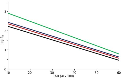
where MW is the molecular weight in daltons. For some types of samples, plots of equation 5 appear as in Figure 2. Here it can be seen that the log k versus S plots are parallel or tend to fan out from each other as %B is reduced. In a case like this, the chromatogram would spread out, with increasing resolution at smaller values of %B, as might be expected from the behavior observed in Figure 1. This kind of sample has been referred to as a “regular” sample. Regular samples tend to be those closely related in structure, such as homologs or isomers. The sample of Figure 2 is a group of structurally related triazine herbicides.
Figure 2: Plot of log k versus %B according to equation 5. Data for a regular sample from reference 5 are triazine herbicides separated on a C18 column in mixtures of methanol-water as the mobile phase.

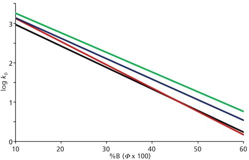
Many, if not most, samples include components that are not as closely related as those just discussed. Such samples vary in core structure as well as in the type and number of functional groups. It is common for plots of equation 5 for these samples to appear more like that of Figure 3. In Figure 3, compounds represented by the black, blue, and green lines behave much like those of Figure 2 in that they are roughly parallel. However, the compound represented by the red line moves relative to the others. At ~45% B, the red and black lines cross, so the two compounds would be coeluted. This is also the crossover point for the red and black compounds; at %B > 40%, the red compound comes out first and at %B < 40% B, it comes out after the black one. In contrast to the expected behavior of Figure 2, the compounds represented by the black and blue lines converge as %B is reduced, so their resolution gets worse, not better, with increased k. Samples in which the slopes of the log k versus %B plots differ significantly are referred to as “irregular” samples.
Figure 3: Plot of log k versus %B according to equation 5. Data for an "irregular" sample from references 6 and 7 are substituted aromatics separated on a C18 column with mixtures of acetonitrile–water as the mobile phase.

The information we gather from Figures 1 and 3 can be valuable guides for LC method development. Figure 1 tells us that we’ll get the “best” chromatographic behavior with 2 ≤ k ≤ 10 (or 1 ≤ k ≤ 20 if the sample won’t fit within this restricted retention range). This is a good general guideline. However, samples that behave as the one in Figure 3 are common enough that we can’t assume that larger k-values (longer retention) will always improve the separation. Sometimes α (equation 2) will remain relatively constant as %B is changed and sometimes it will vary significantly. This tells us that fine-tuning k can be a powerful tool to fine-tune the resolution.
Predicting Retention
Another useful tool that we can use to save experimental runs is to estimate the change in retention (expressed as k) for a selected change in %B. We can do this estimation quite accurately based on two experimental runs that allow us to make plots as in Figures 2 and 3. For example, chromatograms run at 30% B and 50% B would allow us to measure retention for each compound, convert it to k and plot the results as in Figure 2 or 3. Alternatively, we could use equations 5 and 6, along with a single experimental run and knowledge (or guess) of the analyte molecular weights to construct similar plots with a little less accuracy (depending on how many assumptions we make). Equation 6 tells us that a 400-Da compound will have an S-value of approximately 5, which is a convenient number to use as an average or typical S-value for small molecule samples (for example, <1000 Da). From equation 5, we can construct an estimate of the change in k (âk) for a given change in %B (â%B, where â%B = 10% is equivalent to âΦ = 0.1):

Thus for S = 5 and â%B = 10%, we get âk = 10(0.1 x 5) ≈ 3. This is what is often referred to as “The Rule of Three,” where a 10% change in the organic solvent concentration of the mobile phase is expected to change k by approximately threefold. This is a very handy tool for estimating how much retention will change when the mobile phase is modified. I used a similar estimate for the earlier discussion of the effect of a 1% change in %B due to normal variation in the laboratory.
Although I won’t go into detail here (see discussion in Section 2.3.2.2 of reference 2 for more information), we can get plots similar to Figure 2 or 3 if we plot log k versus 1/T, where T is temperature in kelvins. From such data, we can generate a rule of thumb that an increase in temperature of 1 °C will decrease k by 1–2%. This rule of thumb can be useful to help estimate the effect of a change in column temperature on retention and also alerts us to the importance of column temperature control if we want stable retention times.
Conclusions
We have examined the influence of the retention factor, k, on resolution. After we considered the risks (costs) and benefits of various values of k, using Figure 1 as a guide, we concluded that we are likely to get the “best” chromatography and a good balance of costs (time, solvent costs, resolution, and so forth) if we can adjust the chromatographic conditions to achieve 2 ≤ k ≤ 10, or if the sample won’t fit into this retention range, 1 ≤ k ≤ 20. When k < 1, retention tends to be less stable, resolution is very sensitive to small changes in k, and there is more chance of interferences from the unretained materials at t0. When k > 20, run times become excessive and peak heights suffer. When samples won’t fit in a retention range of 1 ≤ k ≤ 20, a gradient is likely a better choice.
We also saw that while it is a general pattern that resolution increases with an increase in k (as in Figure 1 or 2), there are many cases in which the sample components vary enough that changes in relative retention and even peak reversals can be seen with either increases or decreases in %B. This means that even if the sample is eluted in the 1 ≤ k ≤ 20 range, fine-tuning %B can be a useful tool to move peaks around relative to each other.
Finally, we saw that we can further save the cost of experimental runs by estimating the change in retention or k for a specific change in %B or temperature. If two experimental runs are made, such as at 30% B and 50% B for Figures 2 and 3, quite accurate estimates can be made for the change in retention that can be expected with a specific change in %B.
Often if we start method development with a column that generates N ≈ 10,000 plates (1), find conditions that generate 1 ≤ k ≤ 20 for our sample components, and then fine-tune %B for the best retention, we will obtain a satisfactory separation. If this is the case, method development can be a fairly simple process. If we have optimized these two factors (terms i and iii of equation 1) and are not successful, it is time to look for help in term ii of equation 1, as will be discussed in the next installment of this series.
References
- J.W. Dolan, LCGC North Am. 35(3), 170–173 (2017).
- L.R. Snyder, J.J. Kirkland, and J.W. Dolan, Introduction to Modern Liquid Chromatography, 3rd edition (Wiley, 2010), section 2.5.2.1.
- K. Valkó, L.R. Snyder, and J.L. Glajch, J. Chromatogr.A656, 501–520 (1993).
- L.R. Snyder, J.W. Dolan, and J.R. Gant, J. Chromatogr. A165, 3–30 (1979).
- T. Braumann, G. Weber, and L.H. Grimme, J. Chromatogr. A261, 329–343 (1983).
- N.S. Wilson, M.D. Nelson, J.W. Dolan, L.R. Snyder, R.G. Wolcott, and PW Carr, J. Chromatogr. A961, 171–193 (2002).
- N.S. Wilson, M.D. Nelson, J.W. Dolan, L.R. Snyder, and P.W. Carr, J. Chromatogr. A961, 195–215 (2002).

“LC Troubleshooting” Editor John Dolan has been writing “LC Troubleshooting” for LCGC for more than 30 years. One of the industry’s most respected professionals, John is currently a principal instructor for LC Resources in McMinnville, Oregon. He is also a member of LCGC’s editorial advisory board. Direct correspondence about this column via e-mail to LCGCedit@ubm.com

Polysorbate Quantification and Degradation Analysis via LC and Charged Aerosol Detection
April 9th 2025Scientists from ThermoFisher Scientific published a review article in the Journal of Chromatography A that provided an overview of HPLC analysis using charged aerosol detection can help with polysorbate quantification.
Removing Double-Stranded RNA Impurities Using Chromatography
April 8th 2025Researchers from Agency for Science, Technology and Research in Singapore recently published a review article exploring how chromatography can be used to remove double-stranded RNA impurities during mRNA therapeutics production.


