Automated Gas and Liquid Chromatography Retention Time Modelling and Prediction Using Open-Access Molecular Database Structures and Quantitative Structure-Chromatography Retention Relationships

Retention time modelling and prediction software was developed for gas chromatography (GC) and liquid chromatography (LC applications). This open access software incorporates balloon (3D modelling of compounds) and PaDEL (molecular descriptor calculation) as well as support vector machine regression (modelling). To generate models a list of retention times of known compounds is needed together with their molecular structures in simplified molecular-input line-entry system (SMILES) notation. For validation of the models, independent lists of other compounds are used to compare experimental and predicted retention times. The performance of the developed software was successfully demonstrated on three different data sets, including one independent external data set consisting of 507, 291, and 528 compounds, respectively. This software would be useful for the identification of unknown food contaminants and designer drugs in sports doping, and other applications where accurate mass and tandem mass spectrometry (MS/MS) data alone are inconclusive for the assignment of postulated molecular structures.

Retention time (RT) is one of the criteria presented in guidelines for the confirmation of the identity of compounds detected by liquid chromatography (LC) or gas chromatography (GC) systems coupled to mass spectrometry (MS) in fields such as food safety and sports doping (1,2). According to these guidelines, confirmatory methods should be based on target compounds for which standards are available for comparative analysis of RT and fragmentation in (tandem) MS.

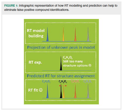
However, in exploratory screenings of samples with separation methods coupled to full-scan accurate mass MS techniques, many signals will relate to compounds for which no standard is available. In practice, without a reference RT and fragmentation information, each accurate mass and elemental composition(s) thereof may be explained by multiple compounds. In these cases RT prediction may help to reduce the number of identification solutions. Aalizedeh et al. (3) modelled and predicted RTs for LC and subsequently used the predicted RTs to help exclude false-positive candidate compounds. The principle of this is represented by the infographics in Figure 1.

In many papers retention modelling and prediction has been performed based on quantitative structure-chromatographic retention relationships (QSRR) (4–6) for a set of compounds measured with LC–MS or GC–MS (3,7–21). It is beyond the scope of this article to review in‑depth all the different software tools and complex chemometric methods described and applied in QSRR modelling and prediction. Basically, for each compound a structure notation (for example, simplified molecular‑input line-entry system [SMILES] format) and retention time are needed. The SMILES is used to calculate molecular descriptors. A selection of molecular descriptors is made based on RT prediction performance. Chemometrics tools are then tested to obtain the best models for prediction by combining descriptors. Finally, in all cases, the validation of a model must be performed on an independent validation set with known RTs, not used for model building (3,7–21).

A major difficulty in using RT prediction in practice is that is that the cited studies (3,7–21), excluding reference 3, have either complex chromatography, a small number of compounds, or not enough information on SMILES and experimental RTs (Supplementary Material S1: Numbers.xlsx). As a result, benchmarking of new developments against previous work is difficult or almost impossible.

In order to make RT modelling and prediction more accessible, new open access software that can model and predict RTs for a wide range of chemically different compounds in GC and LC was developed. Large data sets and simple linear temperature or solvent gradients were used. As an independent validation one-third of all compounds were kept out of modelling and used to serve as substitutes for potential unknown compounds matching the experimental data. Furthermore, an entirely independent external data set from reference 3 was used to benchmark this newly developed software.

Experimental

Obtaining RTs for Compounds for In-House GC, In-House LC, and External LC:

In-House GC:

The retentions of 507 pesticides and contaminants were obtained using GC–MS (Pegasus-4D system, Leco) as described in detail in Lommen et al. (22). Only the first dimension GC retention data (10 m × 0.25 mm, 0.25-µm RTX-CL pesticides column [Restek]) were used. The GC oven temperature was linearly programmed from 60 °C  to 320 °C at 15 °C /min. RTs of GC-stable compounds eluting in the linear temperature gradient were selected, the beginning of the gradient being adjusted to be t = 0 min. RTs and SMILES of all compounds are given in Supplementary Material S2.

In-House LC:

The retentions of 291 compounds were obtained by injecting standards on a Dionex (Thermo Scientific) UHPLC system running a linear gradient separation at a constant flow rate of 0.2 mL/min. The system consisted of a vacuum degasser, a high-pressure binary pump, an autosampler with a temperature‑controlled sample tray set at 7 °C, and a column oven set at 30 °C. Chromatographic separation was performed using a 100 × 2.1 mm, 1.8-µm Zorbax Eclipse Plus C18 column (Agilent Technologies). The mobile phase consisted of 5-mM ammonium formate in 0.02% formic acid (solvent A) and a 90:10 mixture of acetonitrile–water (v/v) containing 5-mM ammonium formate and 0.01% formic acid (solvent B). A gradient elution program started at t = 0 with solvent B at 0% and then increased linearly to 100 % within 40 min, where it was held for 5 min before returning to 0% within 1 min. The injection volume was 5 mL. Peak identities were confirmed by MS (MS method: see Supplementary Material S1). Only compounds eluting during the slope of the gradient were used for modelling; RTs and SMILES of all used compounds are given in Supplementary Material S2.

External LC Data:

Reference 3 is-to our knowledge-the only recent study that includes more than 200 compounds measured with a (more or less) linear gradient separation and provides a ready‑to‑use matrix-containing compound identification, RT, and SMILES format notation. This data was used as an external data source to test and benchmark the software. 511 of the available 528 compounds, that is, all compounds from the linear gradient part of the separation, were used.

Obtaining SMILES for the Compounds: Structural information in SMILES format for nearly all known compounds was obtained from PubChem; care has been taken to use ISOMERIC SMILES (PubChem definition) if the compound conformation requires that (cis/trans; alpha/beta). The developed workflow allows direct manual entry of SMILES as well as automatic retrieval of SMILES using the PubChem compound identification number (CID). For the latter a converted version of PubChem is needed. The publicly available PubChem can be downloaded and subsequently converted using a published PubChem converter (23) following the procedure described in Supplementary Material S3. If SMILES are not available through PubChem they have to be drawn and exported in SMILES format using an external software package (https://cactus.nci.nih.gov/translate/) or obtained through manual internet searches.

Automated Software Events: A detailed description is available in “Details on the procedures done in automation by the software.docx” in Supplementary Material S1. In brief, CalcRetModel uses balloon (24) in-line to transform SMILES to three‑dimensional (3D) (in structure-data file format) SDF files. Consecutively, PaDEL (25) is used in-line to calculate molecular descriptors from the SDF files. At this point there is an option to transform a subset of the descriptor values by a natural log (GC) or by a natural exponential (LC) (See “Details on descriptor modification.docx” in Supplementary Material S1). The data set is sorted and split three ways (Examples in Supplementary Material S4). Two parts are sorted and used for descriptor selection and for generating models using Support Vector Machine Regression (SVM-R) (26). The remaining part is solely used for validation, which is performed after modelling. The developed software automatically selects descriptors and generates slightly differing models. In practice, a high number of models are generated and their prediction outcome averaged to obtain final predicted values. A second program, PredictRet, is also provided in which any new SMILES can be run through the CalcRetModel-generated models to give an averaged RT.

Programming and Hardware: Both of these software programmes are written in Microsoft Visual C++ 2010 and compiled to Windows executables. The compiled binaries are available in the Supplementary Material S5. Calculations have been performed on a hyper-threaded 16-core PC (32 virtual cores; 2.9 GHz; 64 Gb RAM) equipped with a solid-state disc and operated under a Windows (7 or 10) 64 bit operating system. Typically, calculation of 240 models takes about 1–2 days of calculations using 32 cores. In practice, predicting a RT for verification of a new candidate compound using SMILES format takes only a few minutes (Powerpoint manuals of modelling and prediction software modules are supplied in Supplementary Material S5).

Results and Discussion

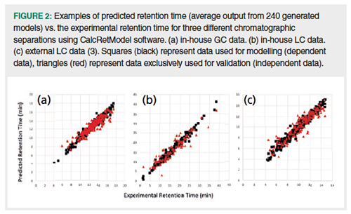
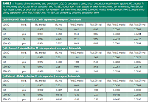
Modelling and Prediction Results: Three different chromatographic separations were used to assess the performance of this retention time modelling and prediction software. Two of these-GC and LC data-were acquired in our laboratory; one LC data set was taken from the literature (3). The results are given in Table 1 and Figure 2. For all three separations the models were validated with a third of the original data set; these validation compounds (red triangles in Figure 2) were not used in modelling and are totally independent.

Modelling and prediction were performed with and without descriptor modification and 3D descriptors (see Table 1) for all three data sets. The RMSEP_val (root mean square error of prediction) values were divided by the effective separation time for the different data sets to obtain a relative value (that is, Rel_RMSEP_val). All three data sets have similar Rel_RMSEP_val values, which indicates that their relative precision of RT prediction is also similar. For in-house data sets (GC and LC), a slight improvement was obtained by modifying descriptors prior to modelling and prediction (See also “Details on descriptor modification.docx” in Supplementary Material S1). Adding 3D descriptors may have a small effect on the external LC data set. Since descriptor modification and adding 3D descriptors may be beneficial, these options were included in the calculations and software.

Averaging RT Output from Multiple Models: Descriptor selection is automated (see “Details on the procedures done in automation by the software.docx” in Supplementary Material S1) for each of the 240 models generated for each data set. Each model is (slightly) different and may perform better for some compounds than for others. Selecting the best performing models may be a biased choice towards those compounds used. It was therefore decided to use all generated models and average the predicted RTs afterwards to remain as independent as possible. If the Rel_RMSEP_val (with descriptor modification and using 3D descriptors) is taken from each individual model (240 total) and averaged and the standard deviations calculated, for the in-house GC, in‑house LC, and the external LC data, respectively, an averaged Rel_RMSEP_val (standard deviation) of 0.0825 (0.0058), 0.0751 (0.0074), and 0.1009 (0.0055) is obtained. Comparison to the values in Table 1 (0.0694, 0.0636, and 0.0897, respectively) shows that an approach in which multiple models are used after which the predicted RTs are averaged decreases prediction errors. Large numbers of models were generated, since this is automatic and just needs computing time.

Benchmarking Using the External LC Data Set: For the external LC data it was reported in the literature that the best R² = 0.887 and the best RMSEP = 0.941 (3) after trying various methods. With this newly developed software approach, an R² = 0.836 and RMSEP_val = 0.99 was obtained.

Comparing Descriptor Lists Between Different Chromatographic Separations: In Supplementary Material 4 a list of descriptors (“Used_descriptors.xlsx”) and the number of times they occur in 240 models is compiled.

In-House GC Data:

All GC models included the descriptors piPC1 (PaDEL Path Count: Conventional bond order ID number of order 1 [ln(1+x)[27]) and MLFER_L (theoretically estimated solute gas-hexadecane partition coefficient [28]). piPC1 is related to ln(nBonds) (See “Details on descriptor modification.docx” in Supplementary Material S1); nBonds (Number of bonds [excluding bonds with hydrogen] [25]) is present in 228 models. Therefore both size, bond order, and theoretical partitioning constant are represented in the models.

In-House LC Data:

All models for the in-house (one‑slope) linear acetonitrile gradient LC data contain CrippenLogP (Crippens theoretical logarithm of the octanol–water partitioning coefficient based on 68 types of atomic contributions [29]) and SpMax2_Bhv (Largest absolute eigenvalue of Burden modified matrix - n 2 / weighted by relative van der Waals volume [3]). The log of the octanol–water partitioning coefficient (LogP) has long been known to contribute to RT modelling of C18-type separations such as those observed here (13). Burden descriptors have been used in prediction of LogP (30). SpMax2_Bhv contains information on atom connections as well as van der Waals volume.

External LC Data:

All models for the external (one‑slope) linear methanol gradient LC data contain CrippenLogP (29), XlogP (another LogP atom-additive approximation method [31,32]) and LipoaffinityIndex (33) (a theoretical modelled measure for hydrophobicity). In contrast to the acetonitrile gradient for in-house LC-data, hydrophobicity fits better as a factor in this methanol gradient.

Comparing LC Descriptors:

Both LC data sets have a high number of compounds and a broad chemical diversity. Both LC data sets have a separation based on C18 columns. Yet the LC data sets show different numbers for how many times descriptors are used in the 240 models. Examining descriptors in both LC data sets already shows differences (“used_descriptors.xlsx”). This may be the result of differences in polarity and solvation by the organic phase in the elution solvents (that is, acetonitrile in in-house LC vs. methanol in the external LC) (34).

Practical Implications of this Approach for GC–MS and LC–MS: To create models for GC–MS and LC–MS, the SMILES and RTs of hundreds of standards are needed. The models obtained are characteristic of a specific standardized chromatography system. If a totally different stationary phase with different chromatographic characteristics is used then the models obtained are no longer applicable and require redevelopment. When using columns with similar separation characteristics, but perhaps different gradients or only different dimensions, it may be an option to calculate RTs using models from this study and then reference their experimental RTs to compounds measured in this study. Predicting RTs (with PredictRet) can be used to help narrow down the number of candidate compounds in identification questions and exclude false positives (3,7–21). For the validation sets of the in-house GC, in-house LC, and external LC data, a retention window of predicted RT ± 2xRMSEP_val will include approximately 93%, 94%, and 94% of the 169, 97, and 170 validation compounds, respectively. A retention window of predicted RT ±3xRMSEP_val will include more than 99% for all three separations. Previously, Berendsen et al. (35,36) modelled the probability of the occurrence of a RT in LC–MS/MS with QSRR and showed that inclusion of chromatographic retention may add significantly to the certainty of identification of unknown and confirmation of known compounds in both tandem- and high-resolution mass spectrometry. Considering that the prediction error with the new software presented here is better, an improvement in identification would certainty be expected.

Conclusion

Open source software was developed for the modelling and prediction of RTs for GC and LC separations. The software runs on a Windows platform and can use multiple processors in parallel. The use of this software is simple and the process is completely automated. This makes it easy to update models if more compounds are added later on. All that is needed as input is enough compounds-described by SMILES and RT-distributed over the standardized chromatographic separation. For in-house GC, pesticides and food contaminants were used. For in‑house LC data, compounds listed as doping compounds were used. The external LC data-the benchmark data for which comparable prediction results were achieved-consisted of emerging contaminants. The compounds used in all three separations may be considered to be chemically highly diverse in terms of polarity and retention behaviour and thus quite challenging for modelling and prediction. It is envisaged that the developed software will be useful to identify unknown contaminants in food and the environment, designer drugs in sports doping, and any applications where accurate mass and tandem mass spectrometry data alone are inconclusive for the assignment of postulated molecular structures.

Acknowledgements

This project is financially supported by the Qatar National Research Fund (QNRF proposal No: NPRP 7-696-3-188) and by the Dutch Ministry of Economic Affairs (project: 1257322801, 1287368201, and 1267333701).

Supplementary Material

All Supplementary Material mentioned in the text is available at: https://doi.org/10.18174/501020. For further information contact arjen.lommen@wur.nl

References

1. WADA Technical Document – TD2015IDCR (2015): https://www.wada-ama.org/en/resources/science-medicine/td2015idcr
2. Guidance document on analytical quality control and method validation procedures for pesticide residues and analysis in food and feed. SANTE/11813/2017 (2017): http://www.eurl-pesticides.eu/docs/public/tmplt_article.asp?CntID=727
3. R. Aalizadeh, N.S. Thomaidis, A.A. Bletsou, and P. Gago-Ferrero, Chem. Inf. Model.56, 1384–1398 (2016).
4. R. Kaliszan, Quantitative Structure-Chromatographic Retention Relationships (John Wiley and Sons, New York, USA, 1987).
5. R. Kaliszan, Structure and Retention in Chromatography - A Chemometric Approach (Harwood, Amsterdam, 1997).
6. K. Heberger, J. Chromatogr. A 1158, 273–305 (2007).
7. H.F. Chen, Anal. Chim. Acta 609, 24–36 (2008).
8. A.G. Fragkaki, A. Tsantili-Kakoulidou, Y.S. Angelis, M. Koupparis, and C. Georgakopoulos, J. Chromatogr. A1216, 8404–8420 (2009).
9. D.J. Creek, A. Jankevics, R. Breitling, D.G. Watson, M.P. Barrett, and K.E.V. Burgess, Anal. Chem.83, 8703–8710 (2011).
10. K. Gorynski, B. Bojko, A. Nowaczyk, A. Bucinski, J. Pawliszyn, and R. Kaliszan, Anal. Chim. Acta 797, 13–19 (2013).
11. T.H. Miller, A. Musenga, D.A. Cowan, and L.P. Barron, Anal. Chem. 85, 10330–10337 (2013).
12. E. Alladio, V. Pirro, A. Salomone, M. Vincenti, and R. Leardi, Anal. Chim. Acta878, 78–86 (2015).
13. R. Bade, L. Bijlsma, J.V. Sancho, and F. Hernández, Talanta 139, 143–149 (2015).
14. K. Munro, T.H. Miller, C.P.B. Martins, A.M. Edge, D.A. Cowan, and L.P. Barron, J. Chromatogr. A1396, 34–44 (2015).
15. C.D. Broeckling, A. Ganna, M. Layer, K. Brown, B. Sutton, E. Ingelsson, G. Peers, and J.E. Prenni, Anal. Chem.88, 9226–9234 (2016).
16. F. Falchi, S.M. Bertozzi, G. Ottonello, G.F. Ruda, G. Colombano, C. Fiorelli, C. Martucci, R. Bertorelli, R. Scarpelli. A. Cavalli, T. Bandiera, and A. Armirotti, Anal. Chem.88, 9510–9517 (2016).
17. A.M. Wolfer, S. Lozano, T. Umbdenstock, V. Croixmarie, A. Arrault, and P. Vayer, Metabolomics 12(8), 1–13 (2015).
18. R.I.J. Amos, E. Tyteca, M. Talebi, P.R. Haddad, R. Szucs, J.W. Dolan, and C.A. Pohl, J. Chem. Inf. Model. 57, 2754–2762 (2017).
19. C. Zisi, I. Sampsonidis, S. Fasoula, K. Papachristos, M. Witting, H.G. Gika, P. Nikitas, and A. Pappa-Louisi, Metabolites7, 7 (2017).
20. Y. Marrero-Ponce, S.J. Barigye, M.E. Jorge-Rodríguez, and T. Tran-Thi-Thu, Chem. Pap. 72, 57–69 (2018).
21. M. Taraji, P.R. Haddad, R.I.J. Amos, M. Talebi, R. Szucs, J.W. Dolan, and C.A. Pohl, Anal. Chim. Acta1000, 20–40 (2018).
22. A. Lommen, H.J. van der Kamp, H.J. Kools, M.K. van der Lee, G. van der Weg, and H.G. Mol, J. Chromatogr. A1263, 169–178 (2012).
23. A. Lommen, Anal. Chem.86, 5463–5469 (2014).
24. M.J. Vainio and M.S. Johnson, J. Chem. Inf. Model 47, 2462–2474 (2007).
25. C.W. Yap, J. Comput. Chem.32, 1466–1474 (2011).
26. C.-C. Chang and C.-J. Lin, ACM Trans. Intell. Syst. Technol.2, 1–27 (2011).
27. R. Todeschini and V. Consonni, in Handbook of Molecular Descriptors (Wiley-VCH Verlag GmbH, 2008).
28. J.A. Platts, D. Butina, M.H. Abraham, and A. Hersey, J. Chem. Inf. Comput. Sci. 39, 835–845 (1999).
29. S.A. Wildman and G.M. Crippen, J. Chem. Inf. Comput. Sci. 39, 868–873 (1999)
30. F.R. Burden, Quant. Stuct-Act. Relat.16, 309–314 (1997).
31. R. Wang, Y. Fu, and L. Lai, J. Chem. Inf. Comput. Sci. 37, 615–621 (1997).
32. R. Wang, Y. Gao, and L. Lai, Perspectives in Drug Discovery and Design 19, 47–66 (2000).
33. R. Liu, H. Sun, and S.S. So, J. Chem. Inf. Comput. Sci. 41, 1623–1632 (2001).
34. B.P. Johnson, M.G. Khaledi, and J.G. Dorsey, Anal. Chem. 58, 2354–2365 (1986).
35. B.J.A. Berendsen, A.A.M. Stolker, and M.W.F. Nielen, J. Am. Soc. Mass Spectrom. 24, 154–163 (2013).
36. B.J.A. Berendsen, R.S. Wegh, Th. Meijer, and M.W.F. Nielen, J. Am. Soc. Mass Spectrom.26, 337–346 (2015).

Arjen Lommen received his Ph.D. in 1990 at Leiden University. After a postdoc period (NMR on proteins) at Radboud University he became the NMR-scientist at Wageningen Food Safety Reserach (WFSR) in 1991. Since then his main focus has changed to metabolomics in GC–MS and LC–MS and writing software in C(++) to perform advanced analysis for metabolomics-type applications with NMR, GC–MS, LC–MS, and GC–GC–MS

Péter Horvatovich received his Ph.D. from the University of Strasbourg (France) in food analytical chemistry in 2001. After two years spent in pharmaceutical industry at Sanofi-Synthelabo (Budapest, Hungary) and one and half year at Bundesinstitute für Risikobewertung (Berlin, Germany), he joined Analytical Biochemistry group at University of Groningen (Groningen, The Netherlands), where has worked for the last 14 years. He is currently associate professor.

Ariadni Vonaparti graduated in 2003 from University of Athens (Greece) with a bachelor’s in pharmacy, where she also completed her M.Sc. in pharmaceutical analysis in 2005. She has spent over 15 years working as LC–MS specialist in the anti-doping field, in bioequivalence studies and research institutes and in 2011 she gained a post-doctoral fellowship in mass spectrometry at the National Hellenic Research Foundation for establishing LC–MS methodologies for identification of new synthesized compounds, metabolomics and lipidomics. She is currently working at ADLQ as Head of the LC–MS section of the Doping Analysis Lab.

Mohammed Ghanim Al Ali AL Maadheed is the chairman of the Board of Trustees of the Antidoping Lab Qatar.

Michel Nielen obtained his Ph.D. at the VU university (Amsterdam, The Netherlands) in 1986. After a career at TNO and in chemical industry at AkzoNobel, he became program manager veterinary drugs at Wageningen Food Safety Research (WFSR). In 2007 he also became extraordinary professor at Wageningen University, focusing on research and development of bioactivity-related multimethods for the detection of chemical contaminants in the food chain. Since 2012, he is principal scientist at WFSR and professor of analytical chemistry at Wageningen University. He has (co-)authored more than 200 peer‑reviewed papers (>8600 citations, H-index 51) covering a wide range of analytical technologies, including mass spectrometry, chromatography, capillary electrophoresis, and biosensors.

Costas Georgakopoulos is a chemical engineer. He was a staff member and director in the Doping Control Laboratory of Athens, Greece, during the period 1988Ð2011. Since 2011, he has been the Doping Analysis Lab Director of the Antidoping Lab Qatar in Doha, WADA Accredited.