Statistics for Analysts Who Hate Statistics, Part VII: Sum of Ranking Differences (SRD)

Comparing methods, models, chromatographic columns, or samples can be achieved with several data analysis methods. We have already explored some of them (clustering, principal component analysis, and desirability functions, for instance). In this seventh installment, we explain a simple and straightforward method: sum of ranking differences.

Comparing methods, models, chromatographic columns, or samples can be achieved with several data analysis methods. We have already explored some of them (clustering, principal component analysis, and desirability functions, for instance). In this seventh installment, we will learn about a simple and straightforward method: sum of ranking differences.

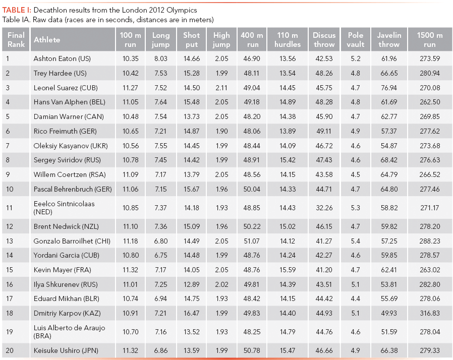
Sum of ranking differences (SRD) (1–3) compares methods or models not based on raw data, but based on ranks. To explain the principle with a basic illustration, one simple example where ranking is applied is sports. For instance, the results of decathlon from the London 2012 Olympics are presented In Table IA. The results for the 20 best athletes in the 10 sporting disciplines, with their scores and the final ranks, are shown.

Instead of classifying the athletes, we classified the sports, to see if any trends were visible in the data, relating some sports to others. For instance, it would seem logical that those athletes that are good in the 100 meters should also be good in the 400 meters or that throwing a discus and throwing a javelin should not be unrelated.

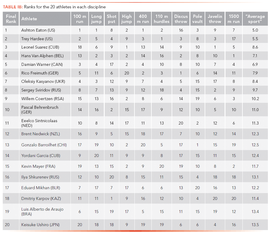
The first step is then to assign a rank to each athlete for each of the 10 sports. The ranks can be seen in Table IB. For instance, the man who ranked first overall (Ashton Eaton) ranked 1st in the 100 meters, the 400 meters, and the long jump. He ranked 2nd in the 110 meter hurdles and high jump, 3rd in pole vault, 7th in the 1500 meters, 8th in shot put, 9th in the javelin throw, and 16th (clearly not his favorite) in the discus throw.

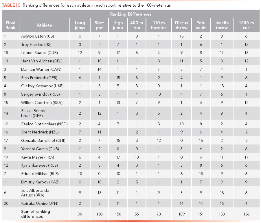
The second step is to choose a reference sport. In our example, we will use the 100 meters as the reference sport. Then the rank obtained by each athlete in every other sport will be compared to the reference sport. As you can see from Table IC, for the gold winner, Ashton Eaton, the "ranking difference" (RD) for the 400 meters and the long jump will be 0 (he won those two events), the RD for the 110 meter hurdles and high jump will be 1, the RD for pole vault will be 2, the RD for the 1500 meters will be 6, and so on. Absolute values are used, because only the distance from the reference is considered. Thus, for the athlete who was the 20th in 100 meter race, the ranking difference in long jump, where he was the 18th, should be RD 2.

Table IC: Ranking differences for each athlete in each sport, relative to the 100-meter run

Finally, for each sport the "ranking differences" obtained by the twenty athletes are added to obtain the "sum of ranking differences" or SRD. The SRD values, at the bottom of Table IC, confirm that an athlete good at the 100 meters should also be good at the 400 meters, because the 400 meters has the smallest SRD value (55) of all nine sports when compared to the "reference sport" (100 meters). Unsurprisingly, the second closest sport is the 110 meter hurdles (SRD 73). The next closest is the long jump (SRD 90), which is understandable when one considers that the same muscles are required for the long jump and short races. At the other extremity of this SRD classification, the sports that are most unlike the 100 meter race are the javelin throw (SRD 153), pole vault (SRD 151), and high jump (SRD 150).

To obtain a scale that would be easier to compare between different problems, the SRD values could be further scaled between 0 and 100 (not shown).

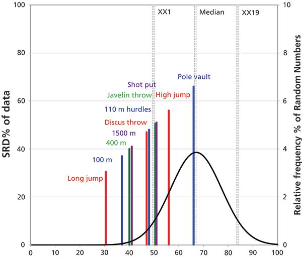
The same SRD ranks could be calculated choosing any other sport as a reference. Another reference sport could have been a fictional "average sport," to see which sport would be most representative of the average performance of a decathlon athlete. For that, the average rank obtained by each athlete for the 10 sports would first be calculated (this is visible in the last column of Table IB). For instance, the gold winner has an average rank of 5.0, while the twentieth best athlete has an average rank of 13.5. Then the ranking differences would have been calculated based on this "average sport" ranking. In that case, SRD values would have shown that the sport discipline that is closest to the "average sport" is long jump (SRD 61), while the sport discipline that is most different from the "average sport" is pole vault (SRD 132). Thus, performance in the long jump is generally a good indicator of overall performance in the decathlon. While the correspondence between the decathlon overall and the long jump is not perfect, there is indeed a tendency showing some agreement (as opposed to the pole vault, where the ranks are completely scrambled). The results are best seen with a figure (Figure 1); the sports appearing on the left side of the Gaussian curve are most similar to the "average sport"; thus the performance of the athletes in these sports should be most representative of the final decathlon ranks. In some cases, the classified objects may appear on the right-hand side of the Gaussian curve, exhibiting "reversed SRD ranking," indicating they are most dissimilar to the reference. Another interesting observation is the clustering of classified objects in this figure: the ranking is not perfectly continuous; rather, groups of sports appear clustered, relative to the reference.

Figure 1: Sum of ranking differences (SRD) ordering of decathlon sports disciplines compared to an "average sport." The x- and left-hand y-axes contain the scaled SRD values between 0 and 100. The Gaussian curve is fitted to the random numbers; their relative frequencies are on the right-hand y-axis.

Now that you understand the principle, let us see one example from analytical chemistry. For instance, SRD was applied in the past (4) to compare chromatographic columns based on the retention of a set of analytes. This could be useful for particular applications where the reference column is inadequate, for instance (a) because one target analyte was eluted with a poor peak shape or (b) because of co-elutions. In the first case, finding a chromatographic column that would provide the most similar retention and separation behavior (but hopefully better peak shapes) is desirable. In the second case, on the contrary, finding a dissimilar stationary phase is desirable. In the report referenced above, 70 columns were compared to the reference column. The first three ranked according to SRD provided the most similar elution profiles to the reference column but with improved peak shapes. Other columns with larger SRD values were shown to provide different elution orders from the reference column and thus would be adequate choices when a complementary method is desired.

A second example is the comparison of methods (chromatographic and computational methods) employed to determine lipophilicity measures (5). Chromatographic retention in the reversed-phase or hydrophilic interaction liquid chromatographic modes is often employed to obtain a measurement of lipophilicity (log P). In a 2015 paper, Andric' and Héberger reported a comparison of 28 different measures of lipophilicity. The results indicated that, although the computationally estimated lipophilicity measures were the best, some chromatographic lipophilicity descriptors approached them. The SRD methodology also allowed discriminating between acceptable and non-recommended lipophilicity descriptors.

Another interesting way to use SRD is to identify outliers (6), which will be the topic of a future article in this series.

For those interested, there are of course many more subtleties to SRD (1–3), as I have only drawn a rough picture of it. Freeware designed by the authors and running on Microsoft Excel or MATLAB is available at http://aki.ttk.mta.hu/srd/.

Acknowledgment

Károly Héberger is warmly thanked for assistance with SRD calculations and helpful comments.

References

(1) K. Héberger, Trends Anal. Chem. 29(1), 101-109 (2010).

(2) K. Héberger and K. Kollár-Hunek, J. Chemom.25, 151-158 (2011).

(3) K. Kollár-Hunek, K. Héberger, Chemom. Intell. Lab. Syst. 127, 139-146 (2013).

(4) C. West, M.A. Khalikova, E. Lesellier, and K. Héberger, J. Chromatogr. A 1409, 241-250 (2015).

(5) F. Andric' and K. Héberger, J. Chromatogr. A 1380, 130-138 (2015).

(6) B. Brownfield and J. Kalivas, Anal. Chem. 89, 5087-5094 (2017).

Past Articles in This Series

Read past articles in this series at www.chromatographyonline.com/caroline-west. Topics include:

1. Collect and Examine Your Data

1. Linear Regression and Quantitative Structure–Retention Relationships

1. Principal Component Analysis

1. Clustering

1. Discriminant Analysis

1. Derringer Desirability Functions.

Caroline West

is an Associate Professor of analytical chemistry at the University of Orleans. Her scientific interests lie in the fundamentals of chromatographic selectivity, both in the achiral and chiral modes, mainly in SFC but also in HPLC. In 2015, she received the LCGC award for "Emerging Leader in Chromatography". Direct correspondence to caroline.west@univ-orleans.fr.