Response Surface Designs Part 1 — Types and Properties

Experimental designs are used in method development and robustness testing and have been discussed in an earlier article.¹ An experimental design is an experimental set-up that allows the simultaneous examination of a predefined number of factors in a predefined number of experiments. Method development is often divided into a screening and an optimization step. During the first step, many factors, potentially affecting the method, are screened to determine the most important factors, which are then further optimized.¹

During screening, so-called screening designs are applied. These designs allow evaluating the effects of a relatively high number of factors in a relatively small number of experiments and were already discussed thoroughly in previous columns.^2,3

In the optimization step, either sequential simplex approaches or response surface designs are applied to further examine those factors found most important from the screening step.¹ Usually, two or three important factors are then optimized further. The response surface design results allow modelling the response(s) as a function of the factors to determine the optimal experimental conditions. When applying these designs, it is either assumed that the optimum is situated in the examined experimental domain, defined by the chosen factor levels, or the maximally feasible domain is examined.

Both symmetrical and asymmetrical response surface designs exist.¹ A symmetrical design forms a symmetrical figure when its experiments are plotted as a function of the factor levels, whereas an asymmetrical design does not when considering an asymmetrical domain of the factors. An asymmetrical design is a design applicable in an asymmetrical domain. Symmetrical designs do not fit well in such a domain.¹ Symmetrical designs are thus used to examine a symmetrical experimental domain, while asymmetrical designs are usually applied in cases where an asymmetrical area needs to be explored.⁴ For example, when optimizing the factors pH and percentage organic modifier in a chromatographic mobile phase, the domain with suitable retention for all compounds can be irregular. In such cases, it is recommended to perform an asymmetrical design to cover the experimental domain well.

In this column, the types and properties of the response surface designs, most currently applied in the context of method optimization, are discussed. The analysis of the design results and the simultaneous optimization of multiple responses, which is often required during optimization with response surface designs, will be discussed in a future column.

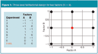
Figure 1: Three-level full factorial design for two factors (N = 9).

Symmetrical Response Surface Designs

Within the symmetrical response surface designs, we consider the three-level full factorial, central composite, Doehlert and Box-Behnken designs as most frequently applied.

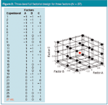
Figure 2: Three-level full factorial design for three factors (N = 27).

A three-level full factorial design contains all possible combinations between the f factors and their L = 3 levels (–1, 0, +1). Thus, N = L^f = 3^f experiments are required to examine f factors in this design. For two and three factors, 9 and 27 experiments, respectively, need to be performed. In Figure 1, the experiments from a three-level full factorial design for two factors are both tabulated and plotted. In Figure 2, a three-level full factorial design for three factors is shown. In both figures, the red experiment represents the centre point. It is often replicated (represented by etc.) to estimate the experimental error in a later data handling.

Figure 3: Central composite design for two factors (N = 9).

Central composite designs (CCD) are the most frequently applied response surface designs. They consist of a two-level full factorial design (2^f experiments), a star design (2f experiments) and a centre point. As a consequence the CCD require N = 2^f + 2f + 1 experiments to examine f factors. The experiments of the full factorial design are situated at levels –1 and +1, those of the star design at levels –α or +α for one factor and the centre point at levels 0 (see Figures 3 and 4). Depending on the α value, two common types of CCD are distinguished. A face-centred CCD (FCCD) with |α| = 1 examines all factors at three levels (–1, 0, +1), while a circumscribed CCD (CCCD) has |α| > 1 and evaluates five levels for each factor (–α, –1, 0, +1, +α). To obtain a so-called rotatable CCCD, the extreme levels of the star design (–α, +α) should fulfil the requirement; |α| = (2^f)^¼. Therefore, |α| is equal to 1.41 and 1.68 for two and three factors, respectively. For two and three factors, a CCD requires 9 and 15 experiments, respectively. In Figures 3 and 4, a CCCD for two and three factors, respectively, is presented. In both figures, the blue experiments represent the full factorial design, the green represent the star design, while the red again represents the centre point.

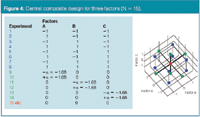
Figure 4: Central composite design for three factors (N = 15).

Doehlert (uniform shell) designs⁵ and Box-Behnken designs⁶ are also regularly applied in optimization. A Doehlert design is characterized by uniformity in space filling, that is, the distances between all neighbouring experiments are equal. For two factors (Figure 5), the design consists of a centred hexagon (N = 7), and for three factors (Figure 6), of a centred dodecahedron (N = 13). The factors are examined at different numbers of levels. For the two-factor Doehlert design, one factor is examined at three and one at five levels, and for the three-factor design, one factor is evaluated at three, one at five and one at seven levels. In Figures 5 and 6, the Doehlert design for two and three factors, respectively, is presented.

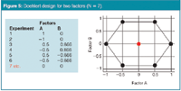
Figure 5: Doehlert design for two factors (N = 7).

A Box-Behnken design requires N = 2f(f – 1) + 1 experiments and the factors are examined at three levels (–1, 0, +1). Thus, for three factors, 13 experiments are needed. In Figure 7, the Box-Behnken design for three factors is shown. A design for two factors is not described.

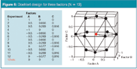
Figure 6: Doehlert design for three factors (N = 13).

As mentioned earlier, for all response surface designs the centre point is often replicated. If done, usually 3–5 centre point replicates are performed.

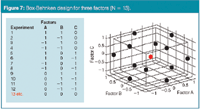
Figure 7: Box-Behnken design for three factors (N = 13).

Asymmetrical Response Surface Designs

D-optimal designs⁷ or the experiments (design) selected with the uniform mapping algorithm of Kennard and Stone⁸ are common types of asymmetrical response surface designs, or designs applicable in an asymmetrical experimental domain. It could, however, be remarked that, when applied in a symmetrical domain, these designs usually have a symmetrical shape. The experiments for these latter designs are selected from a pool of potentially possible experiments in the experimental domain.

When constructing a D-optimal design, first one defines the model to be build from the results. A given model requires a minimal number of experiments, N_min, to estimate its coefficients. Secondly, the number of experiments, N, to be practically performed is defined (N ≥ N_min). This number is user-defined. Then, in the experimental domain, all experiments, forming a grid of potential experiments, are identified (Figure 8). From all combinations of N experiments from the grid points, those where the determinant of X^TX is maximal will form the D-optimal design (red points in Figure 8), with X^T the transpose of the model matrix X.^1,4

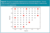
Figure 8: The grid of candidate experiments in an asymmetrical domain. The red points represent the experiments selected for the D-optimal design to examine two factors in nine experiments.

The experiments selected with the Kennard and Stone algorithm cover the experimental domain as uniformly as possible. The experiments are situated as far as possible from each other, by maximizing the minimal Euclidean distance of a new experiment to those earlier selected. The algorithm can be initiated in two ways, either no requirements for specific experiments are defined [Figure 9(a)], or one or some specific experiments are included [Figure 9(b)]. If one experiment is chosen to be included, it is usually the one situated closest to the centre of the domain. If several experiments are, it usually concerns historical experiments that were already executed. The red points in Figure 9 represent the first 9 experiments selected by the Kennard and Stone algorithm. The Kennard and Stone approach involves a sequential selection of experiments, such that the design with 9 experiments is equal to that of 8 to which a 9^th experiment is added. This is not true for the D-optimal designs however, as the designs with 8 and 9 experiments might involve different selections from the grid.

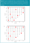
Figure 9: The grid of candidate experiments in an asymmetrical domain. The red points represent the nine experiments selected by the Kennard and Stone algorithm forming a design to examine two factors: (a) without requirements, and (b) with the requirement that the first included experiment is that situated closest to the center of the domain.

Conclusions

In this column, the types and properties of response surface designs, regularly applied in method optimization, were discussed. Most frequently two or three factors are examined in those designs. Designs for more factors are described, but are less frequently applied. We would anyway recommend not to examine more than three factors in a method optimization, because, on the one hand, the number of experiments increases considerably and, on the other, it is not so evident to define the best conditions from such set-ups.

When the factors to be optimized concern only mixture variables, for example mobile phase solvents, then a mixture design approach¹ should be executed and not a response surface design.

From the above, it is also observed that for a given number of factors, say three, different response surface designs can be used. The selection usually depends on the preference of the analyst. Except for the three-level full factorial design, the numbers of required experiments for the symmetrical designs are comparable.

The results of the response surface designs are analysed by building and interpreting polynomial model(s) relating the considered response(s), y, to the examined factors, x_i, for example; y = b₀ + b₁x₁ + b₂x₂ + b₁₂x₁x₂ + b₁₁x₁² + b₂₂x₂². In a future column, this data analysis and the simultaneous optimization of several responses will be discussed.

Yvan Vander Heyden is a professor at the Vrije Universiteit Brussel, Belgium, department of Analytical Chemistry and Pharmaceutical Technology and heads a research group on chemometrics and separation science.

Bieke Dejaegher is a postdoctoral fellow of the Fund for Scientific Research (FWO, Vlaanderen, Belgium) working at the same department on experimental designs and their applications in method development and validation and on the development and data analysis of herbal fingerprints.

References

1. Y. Vander Heyden, LCGC Europe, 19(9), 469–475 (2006).

2. B. Dejaegher and Y. Vander Heyden, LCGC Europe, 20(10), 526–532 (2007).

3. B. Dejaegher and Y. Vander Heyden, LCGC Europe, 21(2), 96–102 (2008).

4. D.L. Massart et al., Handbook of Chemometrics and Qualimetrics: Part A, Elsevier, Amsterdam, (1997).

5. D.H. Doehlert, Appl. Statist.,19, 231–239 (1970).

6. G.E.P. Box and D.W. Behnken, Ann. Math. Stat., 31, 838–864 (1960).

7. P.F. de Aguiar et al., Chemometrics Intell. Lab. Syst., 30, 199–210 (1995).

8. R.W. Kennard and L.A. Stone, Technometrics, 11, 137–148 (1969).