The Perfect Method, Part 4: Controlling Peak Spacing

This is the fourth instalment in a series on method development for liquid chromatography (LC), with an emphasis on developing trouble-free methods quickly. We started out by considering some of the goals we might have and some method development strategies.¹ Next, we selected starting conditions for reversed-phase separations.² This was followed by a discussion of how to control retention for good chromatographic performance.³ This month, we'll consider how to pull apart those troublesome peak pairs.

Getting Retention Right

Last month,³ we were introduced to equation 1:

as a guide for the method development process. Here R_s is the resolution, k is the retention factor, α is the separation factor and N is the column plate number. We looked at ways to adjust the retention factor

by changing the mobile phase strength. (t_R and t₀ are the retention time and column dead time, respectively.) A retention factor of 2 < k < 10 is ideal, but 1 < k < 20 is satisfactory in many instances. There is a regular change in retention with solvent strength for each analyte according to:

where k₀ is the (extrapolated) retention at 0% organic (100% water or buffer), %B is the percent organic solvent in the mobile phase and S is the slope of the plot. The relationship of equation 3 allows us to predict retention for a given analyte based upon just two experiments at different %B-values, because the plot of log(k) versus %B is linear in most instances.

Retention of "Regular" Compounds

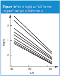
Compounds that have very similar structures, such as homologs, we will refer to as "regular" compounds. These have very similar plots of log(k) vs. %B, as seen in Figure 1 for a sample of nine triazine herbicides.⁴ In such instances, the individual plots tend to fan out, with increasing peak spacing for weaker solvents (lower %B-values). This is what is expected from the fundamental resolution equation (Equation 1) — as k is increased, R_s is increased. However, relative peak spacing doesn't change, so in terms of selectivity, there is little to be gained from a change in the mobile phase strength. As such, a simple change in the mobile phase strength is of little help in pulling apart two peaks that are difficult to separate when samples are all related closely in structure.

Figure 1

Retention of "Irregular" Compounds

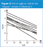
Fortunately, samples comprising entirely "regular" compounds are much less common than those samples whose components differ in functional group types. Such samples we will refer to as "irregular" samples. An example of the retention behaviour of an "irregular" sample is shown in Figure 2 for a mixture of substituted benzoic acids (nitro, chloro, fluoro and so forth) and substituted anilines.⁵ It is obvious that, although the general slope of the plots is similar to Figure 1, the peak spacing for individual pairs of compounds changes dramatically with a change in the mobile phase strength. In several instances, peak crossovers (retention reversals) occur. It is such changes that we can take advantage of, so that by adjusting the %B, we can adjust the selectivity of the separation and pull specific peaks apart. We can also quickly find conditions to avoid, where the lines cross in the plots and, thus, peaks overlap completely.

Figure 2

Taking Advantage of Selectivity

To quantify selectivity, we use the separation factor α:

where k₁ and k₂ are the retention factors of the first and second peak of a given peak pair. If we have retention behaviour as in Figure 2, k-values will not change in parallel, so the α-related term ii of Equation 1 will change, resulting in a change in resolution.

In the earlier discussion of Table 1,² we saw that changing the %B was a great way to change the peak spacing for most samples. Although a change in %B is not the most powerful way to change selectivity, it is very easy, robust and is compatible with UV and mass spectral detectors. Samples that contain analytes with different functional groups, such as those of the irregular sample of Figure 2, will respond well to %B as a tool to change peak spacing. These reasons support our decision to change the %B first in our efforts to finetune the selectivity of a given separation.

The Resolution Map

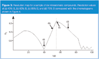
We can use plots, such as Figures 1 and 2, to calculate k for each peak and, thus, α for each peak pair at any %B. Because these plots are on a semilog scale, they can be hard to interpret visually. A more useful approach is to take advantage of the relationship of Equation 1. From our log(k) versus %B plots, we can get values for the retention (i) and selectivity (ii) terms of Equation 1 for any %B. A value for resolution R_s is much more useful than k or α, and this can be obtained by calculating, measuring, or estimating the column plate number N (term iii). If we chose starting conditions with a 150 mm × 4.6 mm column packed with 5 μm particles, the plate number is approximately 10000,² which is sufficiently close for resolution estimates using Equation 1. Now, we can plot R_s versus %B, as shown in Figure 3 for a mixture of six nitroaromatic compounds. This is called a resolution map and is available in the popular retention modelling software packages (for example, DryLab from Molnar Institute, Berlin, Germany, ChromSword from Merck, Darmstadt, Germany, and ACD/LC Simulator from Advanced Chemistry Development, Toronto, Canada).

Figure 3

The resolution map is a plot of the resolution of the least-resolved, or "critical", peak pair at every %B-value. This is illustrated with the simulated chromatograms of Figure 4 for several points on the resolution map of Figure 3. At 40% B [Figure 4(a)], the minimum resolution is near zero and we see that the last two peaks are merged into a single peak. These two peaks pull apart as we move to higher %B-values, as for 50% B in Figure 4(b). The maximum overall resolution is at the apex of the plot at 55% B [Figure 4(c)], where the resolution of peaks 2 and 3 is equal to that of peaks 5 and 6. If we continue to move to higher %B-values, peaks 2 and 3 become the critical peak pair and the overall resolution is reduced [Figure 4(d)]. Note how the retention times (and, thus, k-values) change for the different conditions of Figure 4. So you can see how this powerful tool can lead you quickly to fine-tuned conditions that give the best overall separation — it can save days of trial-and-error experiments.

Figure 4

Other Variables

The resolution map of Figure 3 is for a variation in the %B, and requires only two experiments to obtain the input data. Similar maps can be made for most of the other variables of Table 1. Resolution as a function of column temperature requires just two input runs, whereas changing solvent type, ion pairing reagent concentration, or pH requires at least three runs to calibrate the retention model. The use of retention mapping in method development can greatly speed-up the development process. It can help quickly identify the best conditions for the separation as well as danger regions to avoid.

Table 1: Ranking the variables.

Conclusions

Once we have adjusted the mobile phase strength so that 1 < k < 20, to get the retention times in a region that is likely to give good chromatographic performance, we can move on to the adjustment of peak spacing. Because most samples contain analytes with a variety of functional groups, our samples usually fall into the category of "irregular" samples, as illustrated in Figure 2. When this is the situation, adjusting the mobile phase percent organic can move peaks relative to each other so that we can hopefully find conditions where all the peaks are resolved from each other. The use of Equation 1 allows us to generate resolution maps that will help to identify quickly the conditions for the best separation. Because the resolution map is constructed based upon real experiments, it can provide very accurate predictions of resolution. If the relationships between retention and mobile phase conditions are linear (or log-linear), two experimental runs are required. For more complex relationships, such as retention versus pH, more experimental runs might be required, but the resolution mapping concept works just as well for such variables. Any of the continuous variables of Table 1 (all except column type) are amenable to retention mapping.

"LC Troubleshooting" editor John W. Dolan is vice-president of LC Resources, Walnut Creek, California, USA; and a member of the Editorial Advisory Board of LCGC Europe. Direct correspondence about this column to "LC Troubleshooting", LCGC Europe, Advanstar House, Park West, Sealand Road, Chester CH1 4RN, UK.

Readers can also direct questions to the Chromatography Forum at www.chromforum.com

References

1. J.W. Dolan, LCGC Eur., 20(9), 438–443 (2007).

2. J.W. Dolan, LCGC Eur., 20(10), 504–509 (2007).

3. J.W. Dolan, LCGC Eur., 20(11), 568–573 (2007).

4. D.P. Herman, H.A.H. Billiet and L. DeGalan, Anal. Chem., 58, 2999 (1986).

(5) H. Xiao, X. Liang and P. Lu, J. Sep. Sci., 24, 186 (2001).