Listen to the Data

Volume 18 Number 1
Pages 17-21

A stepwise process helps isolate and identify the cause of a method failure.

One of the most frequent times that we discover a problem with a liquid chromatography (LC) method is when we examine a data set following the analysis of a batch of samples. This month's "LC Troubleshooting" looks at some data submitted by a reader who suspected that something wasn't right with their results. These data give us a good example of how we can examine data for abnormalities and formulate some experiments to try to identify the problem source so we can correct the problem. I have somewhat obfuscated the details so that the reader and company remain anonymous. The sample comprises a pharmaceutical formulation that was being assayed for potency following a particular stress test. A single batch of product was divided into 12 samples, which were then treated in the same manner. For analysis, two subsamples were weighed from each sample, diluted, and injected, for a total of 24 sample injections. The potency was determined by comparing the area response of each injection to the response of a reference standard. The method stipulates that if the two subsamples disagree by more than 1.0% in assay value, the source of disagreement must be investigated. The reader reported that normally these "duplicate" samples agree within 0.5%.

The data I received are listed in the first two columns of Table 1. Each sample is numbered, and the associated letter identifies the subsample (for example, 1a and 1b are subsamples of sample 1). I have noted the absolute difference between the two subsamples in the third column. The abnormality that triggered the reader's inquiry was the 1.41% difference between samples 4a and 4b. This difference exceeded the limit allowed by the method and required that the chemist perform an investigation to identify the source of the problem so that it could be corrected.

Table 1: Percent assay values for individual injections of a pharmaceutical product.

Initial Examination

When I try to solve a problem like this, I like to examine the data in several ways. Often I find that a table of data, such as that of Table 1, makes my eyes glaze over. I do much better with a graphic representation. To get an idea of how atypical the 1.41% difference is, I constructed the frequency plot shown in Figure 1. Here I simplified the data set by "binning" the absolute differences into groups with 0.25% increments, so you can see, for example, that there were five samples in which the difference between injections was 0–0.25%. All the data points except the 1.41% value were <0.75% difference.

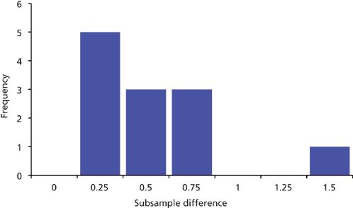
Figure 1: Frequency distribution of subsample differences from Table 1, binned into 0.25-unit increments.

The big gap between the 11 good sample pairs and the one bad one makes the problem pair seem like an obvious outlier. But is there any more quantitative measure of this? One simple technique to test for outliers is the Dixon's Q-test. A test value is calculated as:

For this example, |1.41 – 0.73|/(1.41 – 0.07) = 0.51. The critical value of Q for n ≥ 10 is 0.464 (1), meaning that any test value larger than the critical value is an outlier. Now we have some statistical support in stating that the difference in assay values for sample 4 is an outlier. As I look at the results of the Q-test, however, it looks to me like the 1.41 value isn't very much of an outlier. I checked this by looking at different suspect values using the data set of Table 1, and it is easy to show that the critical value is exceeded only when the suspect value is >1.3%. This says to me that if the current data set is typical for this method, the requirement for differences of <1.0% may be a bit too tight. That is, a value >1.0% will trigger an investigation, but unless it is >1.3%, it is not likely that it can be proven an outlier with the Dixon's Q-test. Such limits should be set as part of the method validation, where large data sets are available and the normal variation of the method can be determined more easily than with the limited data available here.

Digging a Bit Deeper

Sometimes it is useful to examine the data for any trends that might be obvious. An easy way to make a first pass at this is to simply plot the assay values over time. In Figure 2, I have plotted the assay values in order for the 24 injections. There doesn't seem to be any trend to larger or smaller values over the course of the analysis. The variability for the first 12 injections seems to be larger than for the last 12, but these were run on two separate days, so it may be a day-to-day difference as much as anything. The overall variability in the data is shown at the bottom of Table 1 with the percent relative standard deviation (%RSD) of only 0.5%. Considering that many autosamplers have %RSD in the 0.3–0.5% range using reference standards under carefully controlled conditions, it looks to me like this method (including the autosampler) is operating with acceptable precision.

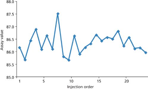
Figure 2: Plot of assay values from Table 1 in injection order.

Although the %RSD is good when comparing samples, I wondered how good the precision was for the same sample with multiple injections. I asked the reader if such data were available, and I was supplied with the data in Table 2. In Table 2, I have shown the results for the original data from Table 1 (4a and 4b), the reinjection data of the same vials (4a-ri and 4b-ri), and the transfer data of the contents to a new vial before reinjection (4a-nv and 4b-nv). I am considering all 4a samples to be equivalent and 4b samples to be equivalent. You can see from the data at the bottom of the table that the variability (≤0.5%) is approximately the same as it is for the between-sample variability for the data of Table 1 (0.5%). This reinforces the conclusion I drew in the previous paragraph that the injection process is working properly.

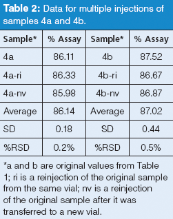
Table 2: Data for multiple injections of samples 4a and 4b.

What Is at Fault?

At this point, we've observed that sample 4 exceeded the maximum allowable difference between subsamples and confirmed that the difference between subsample 4a and 4b is indeed an outlier using the Dixon's Q-test. We have also shown that the results for both samples 4a and 4b have the same level of precision as the remaining samples, so it appears that the problem is not related to the injector. Let's see if we can further narrow the source of the problem to the primary sample 4 or one of the subsamples 4a or 4b. We have enough data now that we can compare the assay values and see if they are consistent.

First, let's compare sample 4a and 4b. With the three "equivalent" injections for each sample from Table 2, we can see if there is a statistical difference between the mean assay value of 4a and 4b. We do this with the Student's t-test that is available as part of the data analysis add-in for Microsoft Excel. We select the two-tailed test because we want to know if there is a difference in the mean values. From the six data points in Table 2, we can calculate a test value of t = 3.19; for a probability α = 0.05, the critical value is t = 2.78, so the Student's t-test shows that there is indeed a significant difference between the mean assay values of sample 4a and 4b. The Excel report (not shown) refines this a bit and indicates that there is only a 3.3% chance that there is not a significant difference in means.

Now we know that samples 4a and 4b are not equivalent. Can we extend the process further and decide if one or both of them are likely to have an error in assay value? We can do the same Student's t-test for sample 4a and sample 4b compared to the remaining samples. One might argue that this is stretching the test a bit, because the larger data set compares variation between samples, whereas 4a and 4b test within-sample variation, but let's ignore that for the moment and see what we get. First, we'll take the data from Table 1 and remove the injections for 4a and 4b, leaving 22 data points. Then we'll take the three data points for 4a and run the t-test comparison, then repeat it for 4b.

When we compare the larger data set to sample 4a, we get a test value of t = 0.76, whereas the critical value is t = 2.07. This tells us that there is no statistical difference between the mean assay value for sample 4a and that of the remaining samples. With sample 4b, the test value of t = 3.20, which exceeds the critical value, means we can conclude that there is a significant difference between the mean assay value for sample 4b and the remaining samples. We may get a better concept of this if we view the data in Figure 3. In Figure 3, I have binned all the assay values from Table 1 into 0.25% increments. As expected, the general form is that of a Gaussian distribution, which would be the case for a large number of points containing random error. The mean (bottom of Table 1) is 86.34, which falls in the 86.5 bin. The value for 4a (86.11) falls in the 86.25 bin, which confirms what we found above: sample 4a is not significantly different than the mean of the remaining 22 values. The value for 4b (87.52), however, falls in the 87.5 bin at the extreme right of Figure 3. With a standard deviation (SD) of 0.42 for the data of Table 1 this means that 4b is 2.8 SD from the mean; for a Gaussian distribution, 99.4% of the values will fall within ±2.8 SD of the mean. Contrast this to the smallest value of Table 1 (85.67), which is 1.6 SD below the mean; 89% of values should fall within ±1.6 SD of the mean, so it is much less likely that 85.67 is an outlier than is 87.52.

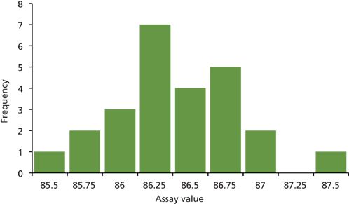
Figure 3: Frequency distribution of assay values for all samples from Table 1, binned into 0.25% increments.

What's Next?

Now that we've identified sample 4b as being an outlier, what else can we do to track down the source of the problem? First, we should eliminate the simple and obvious possibilities. The ones that come to my mind are transcription errors and integration errors. If the analytical balance has a printer attached, check the printer tape to make sure that the weight for sample 4b was transcribed correctly into the calculation of the assay value. For example, the reported weight (not shown) was 100.29 mg; if the decimal values were reversed in transcription from a true value of 100.92, the correct weight (100.92 mg) would change the 87.52 assay value to 86.92, and the difference between 4a and 4b would drop from 1.41% to 0.86%, and would pass the maximum difference test (1.0%) and bring sample 4b within 1.5 SD of the mean. Another possible error is in integration of the peak; double-check that the baseline was drawn properly.

At this point, you may feel that the investigation is complete. We've identified sample 4b as an outlier, and its companion 4a gives a reasonable value. Depending on your laboratory's standard operating procedures (SOPs), you may be able to drop 4b from the data set and use the data from 4a for reporting purposes. Write up your investigation report and you are done. Of course, you should keep your eyes open for similar failures in the future to determine if there is a high enough frequency of failure to merit further investigation.

If you want to investigate further, you need to consider all the possible sources of variation and determine if they are potentially important and if they can be reduced in magnitude. If the sources are independent of each other, the overall coefficient of variation (CV = %RSD/100) can be determined as the square root of the sum of squares of each variable:

where the subscripts represent each independent operation. The operations that come to mind in this instance are sampling, weighing, dilution, mixing, filtration, injection, and integration; there are probably others I've overlooked. Each of these will contribute uncertainty to the overall measurement. Sampling errors reflect how representative the subsamples are. For example, if the sample were granular sugar or a cup of coffee, the primary sample is very homogeneous, so taking a random sample should be fairly representative of the whole. On the other hand, if the sample were a bag of M&M candies, the distribution of the different colours in a small subsample would likely have much more variation. Thus, the homogeneity of the sample and the ability to take a representative sample would influence the sampling step. The variation in weighing could be tested by weighing a fixed standard weight multiple times. The reader did not specify how dilution was done; however, more uncertainty would be expected if a graduated cylinder were used to measure the liquid as compared to preparing the sample in a volumetric flask. Is the mixing sufficient for the concentrated sample and the diluent? Should mixing time be extended, agitation or sonication increased, or other variations in the mixing process be changed to improve the homogeneity of the diluted sample? Does filtering the sample affect the final result? This possible effect could be checked by comparing centrifugation to filtering and seeing if the results were any different. Check the precision of the injector by making replicate injections of a well-behaved analyte. If errors are constant, such as an error of ±0.1 mg on the analytical balance, a fixed volumetric error with a volumetric flask, or ±0.2 μL for sample injection, they can usually be reduced by increasing the sample mass, dilution volume, or injection volume, respectively, to reduce the percent contribution of the fixed error to the total.

Before embarking on a detailed investigation of the method CV, you should step back and consider if it is likely that you will really improve the results of the analysis. A basic principle of statistics tells us that for independent errors, as in equation 2, the largest error will have the most influence on the overall error, that the overall error will never be smaller than the error of the largest contribution, and that the overall error will usually fall between the value of the largest error and twice that value. We determined in Table 1 that the overall method %RSD was 0.5% based on single injections of multiple samples. An autosampler that is operating well should have errors in the range of 0.3–0.5%, so it is unlikely that the overall error can be reduced much below the observed value of 0.5%. In other words, after a brief mental evaluation of the problem, I don't think I'd waste my time trying experiments to reduce the overall error. Instead, I'd stay alert to see if I could correlate future failures to some pattern in the analysis.

Conclusions

Let's review what we've been able to observe about the present problem:

• An error was found when the difference in assay values between equivalent subsamples exceeded the 1.0% threshold.

• By evaluating the difference between subsamples 4a and 4b both visually (Figure 1) and with the Dixon's Q-test, we showed that the difference was indeed an outlier from the remaining samples.

• We also concluded from the Q-test that the 1.0% threshold may have been a bit too tight because, based on the current data set, differences of 1.0–1.3% would fail the test criteria, but would not be proven outliers by the Q-test.

• Based on multiple injections of samples 4a and 4b, we used the Student's t-test to show that there was statistical difference between the mean assay values of the two samples, so they are not equivalent.

• We also used the t-test to find that the assay value for sample 4a fit within the normal range of the remaining samples, whereas sample 4b did not. This test correlated the cause of the problem with sample 4b, not 4a.

• We confirmed the association of the problem with sample 4b by plotting a frequency distribution of the assay values in Figure 3. Sample 4b was clearly at the extreme edge of the plot, whereas the value for 4a was near the middle.

• Before concluding the investigation, it was suggested that we check for obvious errors in numeric transcription and peak integration.

• We mentally evaluated possible sources of uncertainty with the method and concluded that it was unlikely that a thorough investigation of these sources would yield information that would reduce overall uncertainty of the method.

Although the present discussion centred on a specific data set, it illustrates how we can use simple graphic and statistical tools to investigate the failure. We were able to assign the error to a single sample (4b) and demonstrate that its paired subsample (4a) behaved in the same manner as the remaining samples, so it may be possible to use its results to obtain reliable assay data.

"LC Troubleshooting" Editor John Dolan has been writing "LC Troubleshooting" for LCGC for more than 30 years. One of the industry's most respected professionals, John is currently the Vice President of and a principal instructor for LC Resources in Lafayette, California, USA. He is also a member of LCGC Asia Pacific's editorial advisory board. To contact John directly please e-mail: John.Dolan@LCResources.com. To contact the editor-in-chief, Alasdair Matheson, please e-mail: amatheson@advanstar.com

References

(1) J.C. Miller and J.N. Miller, Statistics for Analytical Chemistry (Ellis Horwood Limited, 1984).