Calibration Curves, Part 4: Choosing the Appropriate Model

This is the fourth "LC Troubleshooting" column in a series looking at different aspects of the calibration process for liquid chromatography (LC) methods. We first considered whether or not to force a calibration curve through the origin (x = 0, y = 0).¹ The next stop was a discussion of some techniques to determine the limits of detection and quantification.² Last month,³ we saw how %-error plots could help us visualize possible problems with calibration curves. The present discussion focuses on three different calibration models: external standardization, internal standardization and the method of standard additions. Next month, we will look at the technique of curve weighting.

External Standardization

The use of external standards is the simplest and probably the most common method of calibration for quantitative LC methods. The technique simply compares the detector response between known concentrations of analyte with the response for samples containing unknown concentrations. A calibration curve (also called a standard curve or sometimes a "line") is generated by injecting a series of calibration standards. For well-behaved methods, as demonstrated by validation studies and narrow ranges, for example, ±10% in concentration, a single-point calibration can be used. In this technique, the response (area) for a known concentration of reference standard is calculated (area/concentration) to generate a calibration factor. This value is divided into the area for an unknown concentration and the result is the concentration of the unknown.

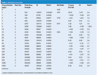
Table 1: Standard curve data.

More commonly, calibrators are prepared that cover the expected sample concentration range and the response of these calibration standards is used to generate a calibration curve. This is demonstrated with the data of Table 1. The data of Table 1 simulate the use of a method for which all the calibrators are injected both at the beginning (data set 1) and end (data set 2) of a batch of samples. Calibrators were prepared at 1, 2, 5, 10, 20, 50, 100, 200, 500 and 1000 ng/mL and injected with the batch of samples. The results are combined in Table 1. Using the data system software or spreadsheet software, such as Microsoft Excel, a calibration curve can be plotted, as is shown in Figure 1. Here, concentration (x-axis) is plotted against response (y-axis). The plot is linear (y = 403.7x – 5.2) and the standard error of y (S_y = 25.1) is greater than the y-intercept, so the curve can be forced through zero (y = 403.7x). (See the discussion of reference 1 for more information on zero-intercept decisions.) This regression equation is then rearranged (x = y/403.7) to calculate the concentration of unknown samples. For example, a sample that generates a peak of 36827 area counts (last line, Table 1) would have a concentration of (36827/403.7) = 91.2 ng/mL. A common sense double-check of the calculation shows that in Table 1, 36827 area counts would fall between 50 and 100 ng/mL, so the result seems reasonable.

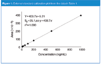
Figure 1: External standard calibration plot from the data in Table 1.

Internal Standardization

External standardization works well when sample preparation steps are simple and the injection volume precision is good. For example, if the sample comprises a pharmaceutical tablet that is weighed, dissolved in an aliquot of injection solvent, filtered and injected with a modern autosampler, external standardization is appropriate. When many sample preparation steps are included in the method or there is a question about autosampler precision, an internal standard can improve the precision and accuracy of a method.

With internal standardization, a second compound, often related to the analyte but never found in the sample, is added at a known concentration to every sample and calibrator. For example, one might pipette 20 μL of a 10 μg/mL solution of internal standard (IS) into 1 mL aliquots of sample and calibrator at the beginning of the sample preparation process. This would mean that each sample would now contain 200 ng/mL of internal standard. If the proper internal standard is chosen, it should track the sample through the sample preparation process, correcting for sample losses because of incomplete extraction, sample loss, or minor differences in reconstitution volume. It is the ratio of the analyte to internal standard that is the critical measurement in an internally standardized method.

The calibration curve data are generated by injecting calibration samples of different concentration that all contain the same concentration of internal standard. The ratio of analyte area to internal standard area is calculated and plotted as the y-value against the concentration of the calibrator. Table 1 shows the internal standard areas and analyte/IS ratios for the same data used for the external standard experiments. The calibration curve is plotted in Figure 2. The y-intercept (0.000051) is less than S_y (0.00011), so the curve is forced through zero. The same unknown used previously (last line of Table 1) generates an analyte/IS ratio of 0.3645. The regression equation is rearranged to x = (y/0.004037), which allows calculation of the unknown concentration of (0.363551/0.004037) = 90.1 ng/mL. This is approximately the same value as that achieved by external standardization.

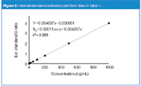
Figure 2: Internal standard calibration plot from data in Table 1.

External or Internal Standard?

Now that we've see the two most common standardization methods for LC, which one should be used? In most cases, precedent will have been set already with similar methods, so the choice should be clear. In other instances, it might not be obvious which calibration type to choose. The simplest way to make the decision is to check the results empirically. Prepare calibrator samples that contain internal standards, as described previously and analyse them. Process the data using both the external standard and internal standard technique. Next, "back-calculate" the calibration samples against the calibration curves and determine the %-error by which each point deviates from the regression line.

Sometimes this is called calculating the residuals. For the data sets discussed previously, the errors for each curve type are shown in columns 7 and 8 of Table 1, with the ratio of the errors in the right-hand column. The results can be compared in several ways. You can compare the results visually at each concentration or the ratio of the errors. Alternatively, you can calculate the average of the absolute values (2.74% for external standard and 1.22% for IS) or the sum of the absolute values (54.8% and 24.5%). In each case, you can see that the internal standard method reduces the error by about two-fold. This supports the use of internal standardization for this method. This suggests that there is some kind of physical sample loss or inconsistent volumetric recovery in the sample preparation process that is compensated by the use of an internal standard. If the results were comparable or the external standard method gave smaller errors than the internal standard method, the simpler external standardization technique should be used.

Method of Standard Additions

When either the external or internal standard calibration method is used, it is usually best to prepare matrix-based standards. This means that the calibration standard is prepared in a solution that represents the sample extract in all ways except the presence of the analyte. For pharmaceutical samples, the blank matrix might be a placebo of the formulation. For bioanalytical samples (for example, drugs in plasma), a drug-free plasma sample might be used. For a pesticide measurement in soil or water, pesticide-free soil or water might be used. By using a matrix-based standard, the likelihood of signal suppression or enhancement by the matrix is reduced. A blank matrix sample is usually run to confirm that there are no interfering peaks present in the matrix.

Sometimes, however, it is impossible to obtain an analyte-free matrix. For example, in the measurement of an endogenous component of blood, such as insulin, it might be impossible to obtain blood without the analyte. Or for the analysis of a waste stream, it might be impossible to formulate a blank sample — that is, the waste stream containing everything except the analyte. When a blank sample cannot be obtained, the method of standard additions can be used to determine the concentration of the analyte in an unknown sample.

A series of calibration standards is prepared at several concentrations. The standards are then added to aliquots of the sample. For the example of Table 1, calibrators were prepared and spiked into sample aliquots to result in samples that contain 0, 1, 2, 5 and 10 ng/mL of added calibrator. Next, the samples are analysed and the results plotted, as in Figure 3. Note that the plot has a significant y-intercept (dashed line in Figure 3); this represents the response for the analyte content of the unspiked sample. To determine this concentration, the regression line is extended to the left until it intercepts with the x-axis (arrow in Figure 3). The x-intercept represents the negative value of the concentration in the unknown sample. This is calculated by taking the regression equation (y = 402.4x + 1055), setting y = 0 and solving for x = 1055/402.4 = –2.6. The negative of this value (2.6 ng/mL) is the concentration of analyte in the unknown sample.

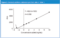
Figure 3: Standard additions calibration plot from data in Table 1.

Summary

We have considered three types of calibration plots this month. You will most commonly encounter the external or internal standard techniques. The choice of the technique can be based upon similar methods in your laboratory, customary usage in your industry, or by empirical testing. Usually, internal standardization, because of its additional complexity, is reserved for methods that require extensive sample preparation, which can result in physical loss of sample in the process. The method of standard additions is usually reserved for cases in which a blank matrix is not available and, therefore, may be rarely, if ever, encountered in many laboratories.

The number of calibration standards used in a method will also vary depending upon the application and the custom for the laboratory or industry. If the calibration plot is linear and passes through the origin, a single-point calibration curve comprising one standard concentration can be justified. However, this technique is often reserved for methods that cover a narrow range in concentrations, such as ±10%. More commonly, calibration standards are formulated at several concentrations that span the expected concentration range of the samples to be analysed. As a general rule, it is best to bracket the concentration range with calibration standards; extrapolation of data beyond the calibration range, while sometimes justified, adds the potential for error to the method.

"LC Troubleshooting" editor John W. Dolan is vice president of LC Resources, Walnut Creek, California, USA; and a member of the Editorial Advisory Board of LCGC Europe. Direct correspondence about this column to "LC Troubleshooting", LCGC Europe, Park West, Sealand Road, Chester CH1 4RN, UK.

For an on-going discussion of LC Troubleshooting with John Dolan and other chromatographers, visit the Chromatography Forum discussion group at www.chromforum.org

References

1. J.W. Dolan, LCGC Eur., 22(4), 190–194 (2009).

2. J.W. Dolan, LCGC Eur., 22(5), 244–247 (2009).

3. J.W. Dolan, LCGC Eur., 22(6), 304–308 (2009).