Calibration

The International Union of Pure and Applied Chemistry (IUPAC) states that "In general, calibration is an operation that relates an output quantity to an input quantity for a measuring system under given conditions". In the International Vocabulary of Basic and General Terms in Metrology (VIM), calibration is defined as an "Operation establishing the relation between quantity values provided by measurement standards and the corresponding indications of a measuring system, carried out under specified conditions and including evaluation of measurement uncertainty".

In chromatography, after performing an analysis, information from the measured signal, for example, from a chromatogram of a sample, is transformed in an analytical result. This action is called prediction. To transform the signal into an analytical result a calibration model is used. The type of calibration considered can be called analytical or methodological calibration and it is performed because the instrument does not directly provide the property (e.g., concentration) the analyst is interested in. Apart from the analytical calibration one can also consider an instrumental calibration to check whether the instrument provides the proper response for an employed standard. The latter type of calibration is not considered in this article.

If only one variable (e.g., peak area), derived from the chromatogram is linked to the analytical result (e.g., concentration), we speak about univariate calibration. When several variables (e.g., areas of different peaks) are related to a result (e.g., antioxidant activity of a wine sample), we call the procedure multivariate calibration. The mathematical relation resulting from the calibration is called the calibration model.

Univariate Calibration

Traditionally in chromatographic analysis, peak area, as information from the measured signal, is related to the concentration of a given substance through a linear regression, resulting in a calibration line (Figure 1). For most quantitative analyses the concentration range is selected in such a way that a linear relation exists with the signal. The calibration line can be described by the following model: y = b₀ + b₁ .x, where y is the peak area, x is the concentration, and bi are the regression coefficients. Classically the regression coefficients are calculated by ordinary least squares (OLS) regression and the coefficients b₀ and b₁ of the calibration line are called intercept and slope, respectively.¹ In general, the regression analysis is performed to study the dependence of the response or dependent variable (y) on the prediction or independent variable (x), a variable that is controlled by the analyst. The variable x is the one that is assumed "error-free" (or with negligible error compared with y) and the y variable, the one that is subject to experimental error.

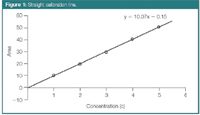
Figure 1

Such a classical calibration curve built with a single result for each standard is called a univariate or a zero-order calibration model. In many instances, univariate calibration models are based on theoretical models such as Lambert–Beer's law for spectrophotometric measurements (in UV detection, absorbance translated to peak area) or Nernst's equation for potentiometric results. The model requires at least two points and can be based on the measurement of a single standard when it is allowed to be forced through the origin (0,0). Often the model is based on the measurement of a number of standards. This allows averaging the experimental error and taking into account an occasional bias in the response.

The signal is assumed to originate only from the compound of interest. In the event of an interference occurring it should have a constant contribution to the signals of all standards and samples. Its contribution is then seen in the intercept (b₀) of the model. When the signal of the interference is not constant in the different samples it is not possible to distinguish between the signals from analyte and interference, and the estimated analyte concentration will be biased (Figure 2). Therefore, in practice in zero-order calibration the collected signal should only result from the analyte of interest, either by using pure standards and samples containing only the analyte or by using a fully selective instrument. In chromatography, it means that the signal (peak area usually) originates from a pure baseline separated peak.

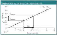
Figure 2

The coefficients of the model can be sensitive to outlying values, especially when the outlier is situated in the highest concentration standard. This value acts as a leverage point and tilts the equation of the line towards the outlying value resulting in biased concentration estimates for the samples (Figure 3). In such situations robust regression methods, such as the least median of squares regression,² minimize the influence of the outlier on the estimated regression coefficients and result in estimates for b₀ and b₁ that are not, or hardly, affected by the presence of the outlying value.

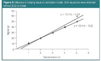
Figure 3

When the standards are measured over a broad concentration range, for example a factor of 1000 between lowest and highest standards, which is regularly encountered in bioanalytical methods, the precision (expressed as variance or standard deviation of replicated measurements) for the different standards is often not constant/similar anymore. This phenomenon is called heteroscedasticity, while homoscedasticity refers to the situation where the variance remains constant.

The latter situation is in fact required to apply OLS regression. When heteroscedasticity occurs weighted least squares (WLS) regression should be applied.³ This is a type of regression in which a higher weight (i.e., more importance) is given to the standards measured with the best precision (i.e., usually those with the lowest concentrations). The problem of heteroscedasticity could also be solved by transforming the variables (e.g., logarithmically).

In some situations, the signal y plotted as a function of x is not linear but curved or curvilinear (Figure 4). It cannot then be properly modelled by a straight line, but a polynomial model is needed. A second-order polynomial, for instance, is represented by y = b₀ + b₁.x + b₁₁.x² and a third-order one by y = b₀ + b₁.x + b₁₁.x² + b₁₁₁.x³ . Higher-order polynomials can also be built. The more complex the model the better it will fit the calibration data. However, from a given complexity the equation will not only represent the general trend of the signal but also the experimental error around this trend. This situation is called overfitting. Such models fit the calibration data very well but this goes at the cost of the predictive abilities of the model. When a model is built for prediction purposes, a compromise has to be found between model complexity and its predictive properties.

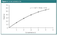
Figure 4

Most calibration models are built to predict the concentration (x) of a sample from its measured signal (y). This means that x has to be inferred from the model for y. This operation is simple for a straight line model, but is somewhat more complex for a curvilinear model. Therefore, sometimes inverse regression is applied. In this approach x is regressed directly on y, resulting in the regression equation x = b_0' + b_1'.y. This type of regression facilitates the predicition of x for new samples, especially from polynomial models. In inverse regression, the error-free x variable is fitted to the y variable that is subject to error.

An example is the modelling of log(molecular weight) or log(MW) as a function of retention time in size exclusion chromatography (SEC) to predict log(MW) values based on the measured retention time of an unknown polymer.⁴ In Figure 5 a third-order polynomial model was used. In multivariate calibration inverse regression is generally preferred to the classical approach.

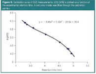
Figure 5

Multivariate Calibration

Multivariate calibration is represented in Figure 6. The objects are samples for which both a chromatogram and a property y (e.g., antioxidant activity, biological activity) are measured. The property y is usually determined with a reference method, for instance, a spectrophotometric method.

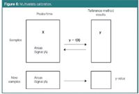
Figure 6

In table/matrix X different measurements from a chromatogram can be collected. It could, for instance, be the peak areas of a number of selected peaks from substances with known activity. It could also be the complete chromatogram, that is table X then contains the measured detector signal (absorbance for instance) for a large number of data points. An additional difficulty when using a complete chromatogram is that the number of time points for every sample in table X should be equal, while the retention times of a given peak in the different chromatograms should be situated in the same table column. Experimentally this is not the situation because of experimental variability, which produces time-shifting between consecutive injections. Therefore, the peaks in a chromatogram need to be aligned first in a data pre-treatment step (Figure 7). Different aligning, also called warping, techniques exist, such as dynamic time warping, correlation optimized warping, parametric and semi-parametric time warping and target peak alignment.

Figure 7

Relating the patterns available in X to the y values is the aim in multivariate calibration. In general, when a vector of results is used for each standard, the obtained model is called a first-order calibration model. When the samples measured in matrix X are subject to, for instance, a time phenomenon (e.g., it is degrading or undergoes a reaction), they could be measured several times as a function of sample age. This results in a series of X matrices differing from the first in the sample age. These matrices (data tables) can be arranged as a cube of data, also called a three-way array. Similar shaped data sets are obtained with hyphenated techniques (e.g., from HPLC-DAD) where chromatograms at different wavelengths are gathered for all samples. Calibration performed on such a data set is called second-order calibration.

In situations where complete resolution of the peak of interest is not obtained, as a result of interferents and univariate calibration is not an option, multivariate calibration can be used. The contribution of the interferents is included in the mathematical model. For this reason the samples used to establish the calibration model should contain the interfering compounds. First-order calibration methods are based on a direct or on an inverse regression multivariate model. The inverse regression is preferred in multivariate calibration. In that context it can be noticed that the notations for X and y are already adapted to that. The independent variable, for example the concentration to predict, is indicated as y, while the response variables are named X, contrary to the situation in direct regression.

The direct multivariate model is a generalization of the classical univariate model. The first-order response (i.e., a spectrum or a chromatogram) is expressed as a function of the concentration of every varying compound in the samples. The model requires the individual signals (spectrum, chromatogram) of all compounds that contribute to the signal of the samples. These signals are often not available, because little is known about the composition of the sample (e.g., herbal extracts, groundwater or wastewater samples).

In the inverse multivariate model y = x.b, the concentration of the analyte of interest or another property of interest (e.g., an activity), y, in the prediction sample is expressed as a function of the response x, a row vector representing, for instance, the chromatogram. The column vector of regression coefficients, b, is previously estimated from a set of calibration samples, for which only the response of interest (concentration of a given compound, activity of sample) must be known. This is also the reason why the inverse model is preferred for multivariate calibration.

The set of calibration samples, unlike in univariate calibration, is much more elaborated and can contain tens or even hundreds of objects. These samples should cover all variability possible in the future prediction samples. The y results for the calibration samples are determined by means of a reference method, as already mentioned.

As for the univariate approach also in first- and second-order calibration different modelling techniques can be used to establish the model. Examples of frequently applied techniques in first-order calibration are multiple linear regression (MLR), principal components regression (PCR), and partial least squares (PLS) regression. Several others that until now have been less frequently used, exist. We will not consider those for second-order calibration. They were discussed earlier in more detail.⁵

In multivariate calibration, often the number of measured variables in the X matrix is larger than the number of calibration samples (objects). The MLR technique cannot deal with such a situation. Therefore, it is accompanied by a variable-selection technique, which selects a number of informative variables, usually much smaller than the number of objects, to include in the model. The PCR and PLS techniques are methods based on a reduction of variables (i.e., the original variables are replaced by a reduced number of latent variables)^6,7 principal components or PLS factors, respectively. These latent variables are then used in the model.

The goal of building a calibration model is to predict the y values of new samples based on their chromatographically determined X-variables. Until now multivariate calibration is mainly used in spectroscopic analysis, where spectra (near-infrared, Raman etc.) are related to the y values. However, the spectral data could easily be replaced by chromatographic. An example, described in the literature,⁸ concerns the prediction of the antioxidant capacity of green tea from the chromatogram by means of a PLS model. The reference method, used to obtain the y values of the calibration samples, was colorimetric.

As for the polynomial models, also in multivariate calibration, the more complex the model the better it will fit the calibration data. Too complex models again result in overfitting. Again, when a model is built for prediction purposes, a compromise has to be found between model complexity and predictive properties. Therefore, during modelling and to select the optimal model, the calibration set of samples is split in a training and a test set, often in the ratio 2/3 vs 1/3, respectively. The training set, which should be large enough to be representative, is used to build multivariate models of different complexity and the test set to evaluate their predictive properties. The (simplest) model with the best predictive properties will be selected and used to predict the y property of future samples.

References

1. D.L. Massart et al., Handbook of Chemometrics and Qualimetrics: Part A, Elsevier, Amsterdam, The Netherlands (1997).

2. P.J. Rousseeuw, J. Am. Statist. Assoc., 79, 871–880 (1984).

3. S. Toasaksiri, D.L. Massart and Y. Vander Heyden, Analytica Chimica Acta, 416, 29–42 (2000).

4. Y. Vander Heyden, S.T. Popovici and P.J. Schoenmakers, Journal of Chromatography A, 957, 127–137 (2002).

5. R. Boqué and J. Ferré, LCGC Eur., 17, 402–407 (2004).

6. D.L. Massart and Y. Vander Heyden, LCGC Eur., 17(11), 586-591 (2004).

7. D.L. Massart and Y. Vander Heyden, LCGC Eur., 18(2), 84–89 (2005).

8. A.M. van Nederkassel et al, Journal of Chromatography A, 1096, 177–186 (2005).

Yvan Vander Heyden is a professor at the Vrije Universiteit Brussel, Belgium, department of analytical chemistry and pharmaceutical technology and heads a research group on chemometrics and separation science.

Ricard Boqué is an associate professor at the Universitat Rovira i Virgili, Tarragona, Spain, working on chemometrics and qualimetrics.

María José Rodríguez Cuesta was a PhD student of Ricard Boqué, who completed a thesis on second-order calibration methods.