Readers' Questions: Calibration

This month's "LC Troubleshooting" looks at two reader-submitted questions regarding method calibration.

One of the parts of being a column editor for LCGC that I enjoy is interacting with readers, primarily by e-mail. I try to answer each reader's question promptly. Some questions have a wider interest to the liquid chromatography (LC) community, so I occasionally pick a question or two to use as the centrepiece of my "LC Troubleshooting" columns. Reader questions also help me keep my finger on the pulse of reader interests so that I can pick topics that will be useful to a wide variety of reader needs. This month I've picked two topics related to method calibration that came in recent e-mail messages. If you would like to submit a question, contact me at the e-mail address listed at the end of this article.

What's the Matter with the Calibrators?

Question: I am running a method to verify that the product we produce contains 100±5% of the label claim of the active ingredient. The method has worked well for our product containing 50 mg of active ingredient. We are just introducing a lower potency product that contains 28 mg of the active ingredient, and I can't get the product to pass the specifications. I weighed out 28 mg of reference standard to check the method and this reference standard will not pass either.

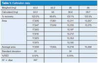
My method calls for making two weighings of ~50 mg of my reference standard and making two standard solutions. Six replicate injections of the first solution (STD1) are made and two of the second (STD2). The response factor is calculated as the average area of the six injections divided by the weight of the standard. System suitability requires that all injections are within ±2% of the nominal amount. I have shown the results of a typical test in Table 1. When I make a lower concentration of reference standard by weighing 28 mg, repeating the injections, and checking the concentration using the response factor, however, I am unable to get the 28 mg standards to pass system suitability. What am I doing wrong? Additionally, the method calls for the two weighings, but after the initial check of the second standard (n = 2), it is not used again. It always seems to agree with the first standard, so why is this required?

Table 1: Calibration data.

Answer: As is my usual practice when reviewing data, I first examine it to see if I can establish any indicators of data quality. One easy way to do this is to look at the repeatability. At the bottom of Table 1 I've shown the average, standard deviation, and percent relative standard deviation (%RSD) for the n = 6 replicate injection sets (as is usual for these discussions, I've rounded the numbers for display convenience). You can see that the 50-mg set comes in at 0.12% RSD and the 28-mg set at 0.23%. Both of these are reasonable and show that the performance of LC system, especially the autosampler and data system, is adequately reproducible. In our laboratory, we typically see ≤0.3% RSD for six 10-μL injections, and these data meet those criteria.

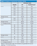
My next step is to examine the individual and pooled results to see if I notice any patterns. I've reorganized the data slightly in Table 2, where the first column of data lists the weighed amounts and the second column lists the amount of compound calculated from the area for each injection using the response factor (RF = 357, bottom of Table 1) based on the weight divided by the average response for the 50 mg, n = 6 sample. You can see that all of the individual 50 mg injections as well as their averages are within the ±2% limit (50.2 mg × 2% = 1.0 mg), so all is well there. However, most of the 28-mg injections and all the averages are outside the limits (28 mg × 2% = 0.56 mg). Because the averages for both 28-mg samples agree (102.1% and 102.6%), it is unlikely to be a weighing error (more on the use of duplicate weighings later).

Table 2: Comparison of results with two calibration methods.

So, what's going wrong here? I suspect that it is a problem with the calibration procedure. This method uses what we call single-point calibration, where a reference standard is made at one concentration and a response factor is determined based on the peak response (area) and the standard concentration. Then sample concentrations are calculated by dividing the sample peak area by the response factor. This is a simple and straightforward technique, but it assumes that the calibration plot goes through zero (x = 0, y = 0). The response factor is simply the slope of the calibration line, and to establish the calibration line, you need two points. One point is the response of the standard and the other is assumed to be zero — that is, zero response for zero concentration — a very logical assumption. However, this assumption must be demonstrated during method validation to justify single-point calibration.

To illustrate the problem, I've assumed that all the weighings at the 50-mg and 28-mg levels are accurate as shown in Table I. By pooling all 16 injections for both concentrations, we can perform a linear regression on the data set. In this case, we get a formula for the calibration curve of y = 346x + 530, with r²= 0.9999. On the other hand, if we only use the 50-mg points and force the origin through zero, we get y = 357x, with r²= 1.0000. It is simple to determine which formula is appropriate for the data set, as was discussed in an earlier "LC Troubleshooting" column (1). In the regression data report for the full data set, there is a value called "standard error of y" (SE_y), which can be thought of as the normal error, or uncertainty around the value of y when x = 0. If the reported value of y at x = 0 is less than the standard error of y, the curve can be forced through zero, and in the present case, this would justify a single-point calibration. If the reported value is greater than the standard error of y, forcing the curve through 0,0 is not justified, and a multi-point calibration is required. In the present case SE_y = 34. In other words, if the calibration line crosses the y axis at 0 ±34, it is within 1 standard deviation of zero and not statistically different from zero, so the use of 0,0 as a calibration point is reasonable. Here, though, the calibration curve y = 346x + 530 tells us that if x = 0, y = 530, which is more than 10 times larger than SE_y, so a single-point calibration is not justified.

To illustrate how much better the data appear when we do a multipoint calibration, I have selected just the second weighings of the 50.2-mg and 28-mg data and used the n = 2 injections of each (four total injections) to generate the calibration curve (y = 342x + 694, r²= 1.0000). I've used this calibration to back-calculate the concentration of each injection, as shown in the right-hand column of Table 2. You can see that the 50-mg data points are about the same as for the response-factor approach, but the 28-mg points all fit within approximately 0.5% of the target values. This is definitely a better choice for calibration of the current method.

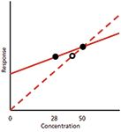
So, why was the problem not noticed with the 50-mg product, whereas it shows up with the 28-mg one? I've sketched a greatly exaggerated calibration plot in Figure 1 with arbitrary slopes to illustrate the problem. With the single-point curve, we have a real data point at 50 mg and an assumed one through the origin that generates the dashed line. By definition, the 50-mg point will be on the line. Any concentration of product that gives a response within ±5% of the 50 mg response will pass the 100±5% specification. Even with the wrong slope of the calibration line, some product concentration variations will pass. I calculate that a product that varied by as much as ±2.5% of real concentration would still appear to fit the ±5% allowance based on the single-point curve. So, if the manufacturing process generated very accurate concentrations (±2.5%), the product would pass specifications. However, product that deviated more than ±2.5% would appear to exceed the ±5% limits. The net result of this condition would be that all "passing" product would be within the specifications and therefore safe to use, but some product that was actually within the ±5% specification would appear to fail and would be scrapped or reworked, adding expense to the manufacturing process.

Figure 1: Hypothetical calibration plots. Dashed line represents 50-mg reference standard and calibration line assumed to pass through the origin (0,0). Solid line represents calibration with 50- and 28-mg reference standards. Open circle shows error in apparent concentration when improper calibration plot is used. See text for details.

When we move to the 28-mg product, however, the story changes. I've drawn the solid curve in Figure 1 to represent the true calibration curve when both the 50- and 28-mg points are used to generate the plot (again, the difference in slopes is exaggerated for illustration). The 28-mg point is shown on this solid line as a solid dot. However, if this same response is plotted on the single-point curve (dashed line), the point is moved to the right (open circle) to fit the curve and gives a reported value that is higher than it should be. This is exactly what we see with the data of Tables 1 and 2 when the response-factor (single-point) approach is taken — the 28-mg values are larger than expected by a little more than 2% (the drawing of Figure 1 greatly exaggerates the difference). With this understanding of the problem, it is not at all surprising that the 28-mg points all fail with the single-point calibration at 50 mg. If another single-point calibration curve were made using 28-mg calibrators, those calibrators would be expected to pass system suitability, and it is likely that at least some of the product batches would also pass specifications for the same reason that the 50-mg ones did with a 50-mg calibration. That is, a single-point calibration can appear to work properly if the test values are close to the calibration point, even if the wrong calibration scheme is used.

I don't know the history of the method or if the single-point calibration was ever validated properly. In any event, when a method is transferred as a pharmacopeial method or an internally developed method, it is always wise to make several concentrations of reference standards over the range of zero to the proposed single-point concentration (and likely to 25–50% higher than the single-point value). Make a calibration curve using all the data points and compare it to a single-point calibration. If they give the same results, easily checked by testing whether the calibration curve can be forced through zero or not, then a single-point calibration is justified.

The final part of the reader's question pertained to the requirement for making two equal weighings of the reference standard and comparing the response of these. Technically, if you are positive that your weighings are always correct, this practice is a waste of time. However, there is a normal amount of uncertainty (error) in the laboratory, and sometimes we just make a mistake. This is the reason for making duplicate weighings — to double-check that a mistake was not made. As a consumer, I am certainly more comfortable depending on a certain dose of a pharmaceutical product if I know the concentration has been double-checked. This is the same reason that duplicate preparations of sample are often called for in an analysis. In some methods, both of the standards are used for calibration. For example, one might have a sequence of STD1, STD2, SPL1a, SPL1a, SPL1b, SPL1b, STD1, STD2, where STD1 and STD2 are the two reference standards, and sample 1 (SPL1) is prepared in duplicate (SPL1a and SPL1b) and each preparation is injected twice. Perhaps all four bracketing standards are averaged to get the response factor for that set of samples. The design of the injection sequence, calibration method, and number of replicates will depend on the analytical method, laboratory policy, and regulatory requirements.

When Should an Internal Standard Be Used?

Question: I'm new to LC and am confused about the difference between an internal and external standard. When should an internal standard be used?

Answer: I discussed the use of various standardization techniques in a couple of earlier columns (2,3), but let's review the highlights here. External standardization receives its name because the reference standard is external to the sample. A single-point standard or a series of reference standards at different concentrations are prepared in a solution, often containing everything that is expected to be in the sample except the active ingredient. That is, known amounts of analyte are added to a placebo or other blank matrix. These are then analyzed using the LC method to establish a calibration curve (also referred to as a standard curve). This curve can be described by a mathematical relationship, the most common of which is a linear fit, y = mx + b, where m is the slope and b is the y-intercept (x = 0). Samples of unknown concentration are then injected and the calibration curve is used to determine how much analyte is present based on the response for the sample, as discussed in the previous example. Additional calculations may need to be made to adjust for the purity of the reference standard, dilution effects, and so forth. Most of the time, external standardization is the simplest way to calibrate a method. It is best when sample preparation is a simple process, such as weighing, filtering, and dilution.

With the internal standard technique, a known amount of a second standard (the internal standard) that is not present in any of the samples is added to each sample. For calibration, a set of reference standard calibrators is prepared, each of which contains the same concentration of the internal standard, but different concentrations of reference standard. Instead of plotting the concentration of analyte versus the response, the concentration ratio of the internal standard to analyte is plotted against the ratio of the area response of the internal standard and analyte. The resulting relationship can then be used to find the concentration of analyte in an unknown sample that contains a known concentration of internal standard.

Sounds complicated, so why go to all this extra work? Internal standardization is especially good when there is a lot of sample manipulation during sample preparation. These might include operations such as liquid–liquid extraction, solid-phase extraction, evaporation to dryness, and other steps where the total volume recovery of the sample may vary. Because the ratio of the analyte to internal standard is tracked, it doesn't matter if only 90% of the sample reaches the injection vial in one case and 80% in the next — such variations are canceled out with the internal standard technique.

Pharmaceutical drug substances (pure drugs) and drug products (formulated product) usually involve simple sample preparation processes, so external standardization is the norm. On the other hand, bioanalytical analysis (drugs in plasma) often comprises many sample preparation steps, so internal standardization is more common for this type of sample. Environmental, biological, herbal, chemical, and other sample types will usually use one or the other of these techniques, depending on the complexity of the sample and how much sample preparation is required.

Conclusions

We have examined some different aspects of calibration. These included the comparison of single-point and multipoint calibration curves, when it is appropriate to force the curve through zero, and when to choose a different calibration method. References 1 and 2 are part of a five-part series of columns about calibration that I wrote several years ago. This series was so popular that LCGC decided to publish it as a stand-alone e-book for ready reference in the laboratory. If you are interested in getting a copy, information is included in reference 4.

John W. Dolan is vice president of LC Resources, Walnut Creek, California, USA. He is also a member of LCGC Europe's editorial advisory board. Direct correspondence about this column should go to "LC Troubleshooting" LCGC Europe, 4A Bridgegate Pavilion, Chester Business Park, Wrexham Road, Chester, CH4 9QH, UK, or email the editor-in-chief, Alasdair Matheson, at amatheson@advanstar.com

References

(1) J.W. Dolan, LCGC North Am. 27(3), 224–230 (2009).

(2) J.W. Dolan, LCGC North Am. 27(6), 472–479 (2009).

(3) J.W. Dolan, LCGC Europe25(6), 316–322 (2012).

(4) J.W. Dolan, Five Keys to Successful LC Methods (LCGC North America e-book, 2013). Available at: http://www.nxtbook.com/nxtbooks/lcgcebooks/lcgc_092013/#/0.