The LCGC Blog: Measuring Quality...

The title will already have many of you shouting at your screen – of course we can’t measure quality. But we can measure uncertainty and build a quality system which helps to produce data which are fit for pupose. Surrogates, Internal Standards, Isotopically labelled Standards, External Standards, Calibrants, QC Samples etc. etc.– our working lives are littered with checks to ensure that our instruments are giving us the correct results. And rightly so.
But do we always use these checks correctly? Do we know what we are checking and why? Indeed, do we know how to design methods/procedures which employ a valid ‘checking regime’, often referred to as a ‘Quality System?’ Let’s find out.

It’s important to point out that different laboratories call calibrants, blanks, recovery and quality check samples different things - so beware of semantics. Also beware that different industries and applications have different regulatory Quality requirements - for example a hospital toxicology lab will have a different empirical approach to control the quality of data produced to an environmental laboratory who in turn will differ from a research and development laboratory etc.
All of this being said – we all strive to accomplish some very basic checks which can be summarised as follows;

How much analyte do I extract from each sample?

• How much of the in-tact analyte reaches the detector on repeat injections?
  
• What is the instrument response to the analyte from each sample?
  
• Are any co-extractants or matrix components likely to change the instrument response to my analytes?
  
• Are instrument artefacts contributing to a change in the response of the instrument from each sample?
  
• Is the response of the instrument changing over time?
  In citing the above list I’ve made some assumptions, such as the instrument has been proven to be producing data which is fit for purpose (using OQ/PV and System Suitability tests). It’s also necessary to point out that there are errors associated with sample extraction and analysis which are inherent within the process (often called Random Error) and other errors which are avoidable and are due to controllable variables within a method (often called Systemic Error), and both of these errors must be measured within our quality system and a tolerable / acceptable level of uncertainty defined. These things are done during method development and validation.

So let’s consider some of the points in the list above with a ‘chromatographers perspective’ to see how our quality system and analyses are linked and to make sure we are clear on why we do what we do in order to generate results and demonstrate that they are fit for purpose.

The efficiency of extraction of an analyte from a matrix, or the processing of a sample to prepare for analysis, will obviously depend upon the chemical nature of the analyte and matrix, and will by definition, vary as the sample matrix varies. We need to account for differences in the efficiency of analyte extraction due to changes in the sample matrix on a sample by sample basis, as well as simultaneously accounting for matrix (co-extractant) effects on the instrument response. Most notably in modern times, this means accounting for the way in which matrix components either supress or enhance the degree of analyte ionisation, and hence response, in LC-MS and GC-MS experiments.

Typically this is done using ‘surrogates’ which are introduced into the analysis at the earliest stage possible and which have the following general properties;

• Chemically similar to the analyte(s) of interest
  
• Behave similarly during extraction and sample preparation and suffer similar signal suppression or enhancement as the analyte(s)
  
• Can be chromatographically or spectrometrically resolved from the analyte(s) of interest
  
• Do not interfere with the instrument response to the analyte(s)
  The list is comprehensive and often the equivalence of the surrogate and analyte are implied rather than being empirically demonstrated. In some cases surrogates are added at a constant concentration to samples, in others, the concentration of the surrogate is matched to the expected concentration of the analyte in order to assess matrix or instrumentation concentration effects.

One must be quite clear on how to assess the surrogate response and the limits within which the surrogate response is satisfactory. How does one derive ‘acceptable’ range for surrogate recovery? Typically this will be guided by the laboratory quality system, regulatory requirements and/or by statistical analysis during method development and validation. How were your surrogate recovery limits derived?

One then needs a ‘decision tree’ to describe the process for handling outliers; high recoveries may not be considered an issue for a limit test in which the analyte is below the reporting level, however a low recovery needs action and very low recoveries may render the data unusable? Do you adjust analyte results based on the surrogate recovery (i.e. extrapolation)? Is this valid; has this process been validated; are you sure about the equivalent behaviours of surrogate and analytes during extraction and MS analysis where appropriate to make this extrapolation? You need to be very sure.

There are methods which use isotopically labelled surrogate compounds which are spectrometrically resolved from the analytes of interest. It must be demonstrated that the use of these specie do not enhance or supress the analyte signal as it varies in concentration relative that of the surrogate.

Further, one needs to consider carefully at what point the surrogate is added to the sample; if added to the first solution created from the sample (i.e. in which the solid sample is dissolved for example), or directly to the diluted liquid sample, is it established that the analyte(s) does not undergo any binding or intermolecular affects which would affect the degree in which the analyte is liberated into solution in its ‘free’ state. Protein binding of analyte in bioanalytical science is a primary example here but there are many others involving chelation etc. Further, if one attempts to add surrogate to a solid sample, how can one assure the homogeneity of surrogate distribution during sub-sampling etc. This is a very broad topic and beyond the scope of our considerations here – however the crux is deciding at which point the surrogate is added to the sample and whether this is then ‘representative’.

Often a ‘Matrix Spike’ is evaluated, which contains the analytes at an appropriate level spiked into blank matrix, which is subjected to full analysis to assess potential interference from matrix components during both the extraction and analysis phases of the method. Unfortunately matrix spiking cannot be performed on each individual sample and variations in the sample matrix between samples can render this exercise meaningless.

In any analysis, we also need to model the instrument response to the analyte and check the reproducibility and instrument drift over time in order to establish the validity of our data.

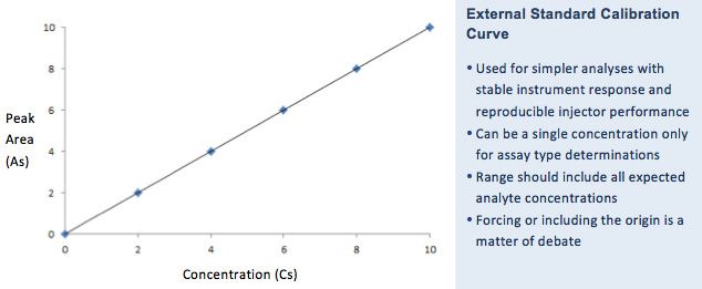
To ‘calibrate’ instrument response, some methods use external standard quantification in which standard solutions of analyte at a single or multiple concentrations are measured to establish a simple model of analyte response v’s concentration. Single level calibration is typically used when the expected analyte concentration is at a single fixed value (assay) and multi-level calibration when the analyte response will vary over time. The number of calibrant levels and the mathematical modelling of the response vs concentration curve will be guided by local and regulatory quality requirements, but a satisfactory range of calibrants should be used to cover the likely range of analyte concentrations and the instrument response curve is typically modelled using linear or polynomial regression. Typically, one would need to assess the inherent error in the regression model by carrying out statistical analysis to assess the sum of squared residuals (SSR) and determine the ‘standard error’ as well as determining the goodness of fit using the coefficient of determination (R2). The use of the coefficient of determination alone is often not considered to be rigorous enough as it can produce misleading results which may, for example, indicate a satisfactory linear fit when the response is in fact polynomial. Decisions such as whether to include or force the regression line through the origin are also a matter of debate and will again depend upon local policy, the use of blank samples, the limits of detection of the method and several other factors.

A question which is often pondered in our laboratory is; ‘do we make up the instrument calibration solutions using blank sample matrix, and are the calibrants subjected to extraction in the same way as the samples’. I would suggest that you consider this point carefully and relate this to your own analyses. Are your calibrants measuring absolute instrument response or are they a measure of the signal generated by a sample which has been subjected to the whole of the analytical process. The difference is very important and fundamental to the quality regime to which you work and how the data produced are handled.

This ‘external standard’ calibration model will work only when the instrument reproducibly introduces fixed volume aliquots of sample into the system and there is no mechanism by which the response of one sample specie can influence the instrument response with respect to another. If there is any doubt about the reproducibility of sample introduction, then an Internal Standard may be used, which would have similar properties to those of a surrogate compound listed above.

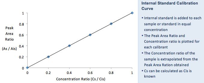
Typically the internal standard is added to all samples (standards, unknowns, QC’s etc.) at a constant concentration. This produces an extra peak within the chromatogram which is used to ‘normalise’ the instrument response – i.e. the calibration curve is constructed using the peak area ratio of analyte to internal standard against the corresponding concentration ratio. The peak area ratio for the analyte in the unknown can then be used to find analyte concentration as the concentration of the internal standard added to the sample is also known. Response factors (RF) are used for the determination of sample concentration;

where: As = Response for the analyte, Ais = Response for the internal standard, Cis = Concentration of the internal standard, Cs = Concentration of the analyte to be measured

Again, it is important to consider how the system may respond differently between the analyte(s) of interest and the chosen internal standard. There are many considerations in this regard but some you may like to ponder include:

Relative volatility of the analyte and internal standard (especially important is assessing analyte losses in GC sample introduction)
The degree to which the compounds may participate in secondary (unwanted) interactions – adsorption to free silanol species of the inlet liner for example
Response per unit analyte of the detector - do the analyte and internal standard response follow similar models – it would be no good having an internal standard with a quadratic response over a concentration range when the analyte response is linear
Does the inclusion of internal standard in any way interfere or influence the detectability of the analyte(s) – ion suppression or ion enhancement would be the obvious examples in LC-MS analysis
One needs to very carefully consider the properties of the internal standard prior to adoption and thorough validation is recommended.

Often, the absolute response of the internal standard is used to assess instrument drift within an analytical campaign, a limit being set for the acceptable drift in response (area ratio). This is a good on-going monitor of drift in system response, however most Quality systems will insist upon the use of Quality Control samples. These are standards, which may be constructed in the matrix of interest and subjected to the full extraction and analysis procedure, which assess the ‘drift’ of a method over time. The determined concentration is compared to the nominal value and must match within a specified tolerance level, which again is defined by local quality systems, regulatory procedures or via statistical analysis during method development and validation. Again one must have a well-defined protocol which describes how data sample data are handled should out of specification QC results be obtained – especially regarding the re-analysis of samples after further within –specification QC checks are performed.

If the analytical system is known to drift over time, for longer campaigns, the instrument may be partly or fully re-calibrated over the course of an analysis. Further, the model for this re-calibration or indeed for the actual determination of sample concentrations differs greatly between laboratories, quality systems and regulatory bodies.

For example, the calculation of sample concentration may use the calibration curve at the beginning of the analysis, or may be based on the average of calibrants either side of the sample of interest (sometimes called ‘bracketing’)or on an average of all calibrants determined across the whole analysis. It is fair to say that there is no right or wrong way of determining the sample concentration – only that the calibration model should correctly account for any drift in instrument response with time. Does your calibration model achieve this??

One should, from time to time, pause to ponder why your analyses are designed as they are and wonder if the quality system model being used is appropriate – or as is sometimes the case – overly complex or cautious and therefore the cause of wasted time. If this were not the case – would the concepts of Quality by Design find so much interest in modern analysis? Whatever the case, we should be fully aware of what aspect of ‘quality’ is being assessed by which of the different solutions we inject and measure.

For more information – contact either
Bev ([email protected]) or Colin ([email protected]).

For more tutorials on LC, GC, or MS, or to try a free LC or GC troubleshooting tool, please visit www.chromacademy.com