Comparison Techniques for HPLC Column Performance
This article investigates the different methods that can be used to compare the performance of liquid chromatography (LC) columns to assess the advantage of using them at high pressures and/or high temperatures. The main focus is on the kinetic plot method. This method, which is based on two simple equations, allows the user to transform the more common Van Deemter curve into a curve describing the ultimate separation speed as a function of the required plate number, or the required peak capacity or the required resolution.
When developing a chromatographic method, chromatographers are often required to determine the best column and operating conditions to address the problem at hand. With so many columns and operating conditions to choose from it is often a challenge to choose the optimum column parameters (e.g., particle size, column length, column internal diameter, etc.) and optimum operating conditions (e.g., mobile phase components, buffers, flow-rates, temperature, etc.).
For most chromatographers, analysing HPLC column performance consists of measuring the following four key performance parameters: the column efficiency [height equivalent theoretical plate (HETP) or H], which is a function of the mobile phase flow-rate; the column permeability, K v0 (or pressure drop), the retention capacity (k value); and the column selectivity (α) for important pairs of analytes. Whereas, the former two essentially reflect the packing quality and the mass transfer kinetics of the column, the latter two essentially depend on the dimensions and the chemistry of the stationary phase.1 Although the overall column quality is also determined by other factors, such as lifetime, chemical inertness and mass loadability, this article will focus on the first four parameters (H, K v0 , k and α) because these generally apply to all separations than the latter three, which depend strongly on the chemistry and the economics of the application.
Effective Performance (Absolute Plots)
Traditional column comparison techniques: In a typical performance report or research paper, the main column performance parameters (H, K v0 , k and α) are often treated and discussed separately. Figure 1 shows such an example. The column efficiency is usually represented by the column Van Deemter curve [Figure 1(a)]. To investigate the pure column performance, the reported plate height values should preferably be corrected for the extra-column band broadening because these features only detract from a fair column comparison, but are particularly important for the smaller particle columns that are being used today.
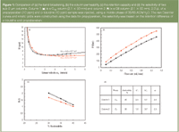
Figure 1
The column permeability is usually assessed from a plot of the column pressure P (preferably also corrected for the extra-column pressure-drop) versus the flow-rate or the interstitial-, the superficial- or the t 0 -marker velocity [Figure 1(b)]. The retention capacity is usually represented as a plot of ln k' versus the fraction of organic modifier (φ) for one or more test components [Figure 1(c)], while the information regarding the column selectivity is usually contained in a table listing the retention factor ratios of close-eluting pairs of components [Figure 1(d)].
The example data shown in Figure 1 have been obtained by comparing two different particle types (similar sub-2 μm size, but bonded with different stationary phases, C8 and C18). Each particle type was evaluated by testing two purchased columns.
Most of the main performance parameters considered in Figure 1 are subjected to a trade-off. Column efficiency and column permeability make a good example. Their trade-off is best imagined by comparing an open-porous monolithic column (lower flow resistance but higher plate heights) with a sub-2 μm particle packed column (higher flow resistance but lower plate heights). Another example of this trade-off is the choice between the two particle types considered in Figure 1. Figure 1(a) shows that the C18 column has a lower plate height in the C-term region of higher velocity (red data points) while Figure 1(b) shows that this same column has the disadvantage of having a substantially lower permeability (higher pressure drop). Which one of the two support types provides the best trade-off between permeability and plate heights is difficult to tell, especially because the answer depends on the plate number needed for the application [vide infra, Figure 3(b)]. Neither the Van Deemter curve in Figure 1(a) nor the pressure–flow-rate curve [Figure 1(b)] tells you which column would be the best choice for a particular separation.

Keynotes
There can also be a trade-off between permeability and retention capacity. This can again be best illustrated by comparing reversed-phase (RP) monolithic and packed columns. An open-porous monolithic column will certainly offer a higher permeability, but might, because of its lower phase ratio, lead to a reduced retention capacity. Thus, to increase the retention capacity it may be necessary to use a more viscous mobile phase (i.e., with a higher aqueous fraction). Another example is the temperature trade-off between the higher retention capacity and higher C-term band broadening of an ambient temperature operation versus the lower C-term band broadening and often lower retention capacity of a high-temperature operation.
Without guidelines on how these trade-offs should be made, column performance comparisons can seldom go further than just making a qualitative statement of the pros and the cons of the different systems being compared. The approach that is usually adopted to go beyond this qualitative comparison is to compare the efficiency, resolution and analysis time of two representative chromatograms, one obtained with a reference system (standard column and standard operating conditions) and one with the new system (new column and/or new operating conditions). These chromatograms are then considered as the ultimate proof of the supposed superiority of this new system. However, the reference system is in many instances used under non-optimized conditions so that the claimed gain in separation performance usually refers to a specific set of conditions. This approach is sometimes used by manufacturers to show that their column is superior to another column and is not a fair comparison.
The kinetic (absolute kinetic plots): A straightforward, practically and economically highly relevant trade-off criterion wherein the individual importance of the four major column performance parameters shown in Figure 1 are properly weighted is the minimal analysis time needed to obtain a given efficiency, or resolution or peak capacity. As has been demonstrated by Desmet et al., this minimal analysis time can be calculated in a very straightforward way, without the need for any computerized optimization algorithm, by simply rearranging the data in a measured Van Deemter curve and the value of the column permeability (K v0).2 This approach is the essence of the kinetic plot method of comparison.
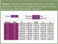
Figure 2
The practical implementation of this rearrangement is illustrated in the spreadsheet table in Figure 2 and is based on the two following simple equations, translating each data couple in a series of (u0, H)-data into a new series of t0-time versus N:

The quantities between brackets are obtained experimentally. The u0- and H-values vary from row-to-row in the table in Figure 2, while the viscosity value (η), the available column inlet pressure (P) and the column permeability normally remain constant throughout the table. While the column permeability (Kv0) is experimentally fixed, the values of ΔP and η can be chosen more freely, but it should be obvious that the most practically relevant system comparison is that where each system is represented by its proper mobile phase viscosity and its proper available maximal pressure drop.
Figure 3 shows the graphical representation of the data rearrangement determined by Equations 1 and 2. As can be noted, each (u0, H)-data point coming from Figure 3(a) — the same data as in Figure 1(a) is transformed into a unique data (t0, N)-data point in Figure 3(b). The outcome of the optimal trade-off between permeability and plate height can now be seen at a glance, for each possible plate number required. The support type with the lowest C-term band broadening (red data) can only be expected to provide superior separation speeds for separations having a t0-time of less than 0.5 min (total analysis time around 5–8 min), while the black data support should be preferred for all applications requiring a higher separation efficiency. Of course, this result assumes that the packing material (support) can be packed as effectively in a column that is shorter or longer than the tested column, but this assumption is also true for any column comparison discussion based on a Van Deemter-curve and a bed permeability.
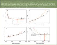
Figure 3
To really grasp the transformation between the Van Deemter-curve and the kinetic plot in Figure 3(b), it is important to realize that each data point of the kinetic plot relates to a separation performed at the maximal pressure (Equations 1 and 2 are used with a fixed, maximal ΔP). Because each data point of the Van Deemter curve relates to a different velocity, it is, therefore, transformed into a separation performed in a column with a different length. Hence, whereas in a Van Deemter curve the pressure varies from point-to-point and the column length is constant, the opposite is true for a kinetic plot curve: the pressure remains constant, while each data point refers to a different column length. As low velocities allow for the use of long columns, it should be obvious that the data points coming from the B-term dominated region of the Van Deemter curve transform into the long analysis time and high resolution end of the kinetic plot (where long columns are needed), while the data points originating from the C-term dominated region transform into short analysis time and low resolution data points (left hand side of plot). In Figure 3, this transition can easily be visualized by following the position of the numerated points.
Because each row in Figure 1 relates to a given N value, it is straightforward to combine this value with the corresponding plate height value to obtain the corresponding column length. The column lengths obtained are plotted in Figure 3(c), providing at a glance all the optimal column lengths needed to achieve any of the possible required plate numbers.
The kinetic plot in Figure 3(b) comprises the complete performance potential of the two tested supports. Another useful data representation format is one where the y-axis values (t0) are divided by the square of the corresponding N-value. Plotting the t0/N2-values obtained as a function of N [Figure 3(d)] offers two major advantages.
Firstly, the y-axis is compressed, allowing for a better resolution between the different curves, and secondly, the curves now go through a minimum at an N-value that corresponds to the velocity where the Van Deemter-curve goes through its minimum (cf. the position of point number 3). This is the point (marked by the optimal plate number value N opt ) where the support is used under its kinetically most advantageous conditions (i.e., in a column that is exactly long enough to reach the optimal mobile phase velocity at the maximal available pressure). In other words, this is the point where the support reaches its so-called Knox and Saleem3 limit line.1 The advantage of the t 0 /N 2 versus N-plot is that it automatically reveals the N-value for which this limit is reached [Figure 3(d)]. If N opt is larger than the actual required plate number, one should try to switch to structures with a smaller feature size (but with the same packing quality), whereas the opposite holds true if Nopt is smaller than the required plate number.
Plots of time versus plate number to compare different chromatographic support morphologies or different physicochemical operating conditions have been used since the early days of chromatography. In 1965, Giddings already presented such a plot to compare the performance limits of LC with those of GC4 on a system-independent basis. Later Knox3 and Guiochon5 used the same approach to compare the performance of packed bed columns with open-tubular columns. In 1997, Hans Poppe proposed to plot t 0 /N versus N instead of t 0 versus N.6 Halasz et al.,7 also devised a method to directly compare columns with a different support morphology. This approach uses an equivalent sphere particle diameter based on the measured column permeability. The obtained plots, however, have no direct relation to the kinetic performance of the tested columns and overestimate the advantage over very open-porous systems such as monolithic columns.
The kinetic plot method provides an addition to the work of Giddings, Knox and Poppe in the sense that the optimal kinetic performance curves presented by these authors were obtained through modelling and computer optimization, whereas the use of Equations 1 and 2 now allows every analyst to establish a kinetic plot for his/her own tested column application and for his/her own specific application.
Once all t 0 - and N-values in the spreadsheet table (Figure 2) are known, it is quite straightforward to use the values of the phase retention factor k' and a measured selectivity factor to calculate the corresponding total residence time [tR = t 0 (1+ k')], the effective plate number [Neff = Nk'2 /(1+k')2 ], the isocratic peak capacity and the resolution Rs. As is illustrated in the schematic representation in Figure 4, plots involving these quantities can be used to extend the trade-off between column efficiency and permeability by also including the retention capacity (plots involving tR and Neff) and even the column selectivity (plots involving Rs).
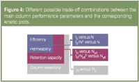
Figure 4
Figure 5 gives an example of the latter. Because the C18-bonded particles provide a higher selectivity for the analytes propylparaben and o-toluidine than the C8-bonded particles [Figure 1(d)], it is not unexpected to find that the range, wherein the C18-bonded particles are beneficial, is even broader in the resolution kinetic plot than in Figure 3(b) and (d), where only the separation kinetics were taken into account and not the selectivity of the supports. Therefore, the type of kinetic plot shown in Figure 5 provides a more complete image of the real chromatographic quality of a tested support. The downside of this "completeness" is that the inclusion of the selectivity parameter makes the plot less general and much more application specific, but this might in many instances just be an advantage.
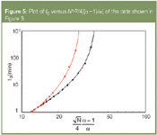
Figure 5
Intrinsic Performance (Reduced Plots)
Reduced plate height plot: Apart from the absolute column performance, it is also customary to look at the dimensionless performance of the system. This dimensionless performance is usually made to assess the intrinsic quality of a column, that is to find out how far the column packing is away from the best possible packing (cf. Knox' theoretical "yardstick"8 ) and whether more effort should be spent on improving the packing homogeneity or not. The use of dimensionless performance parameters dates back from the work of Giddings9 and allows the effect of the particle (or skeleton) size on the band broadening and the column permeability to be filtered out.
Although this approach is indispensable for any thorough column study (it offers an in-depth understanding of the different parameters that contribute to the band broadening and provides a universal measure for the flow resistance), one should be cautious of the fact that the obtained A-, B- and C-term constant depends directly upon the value of the employed mean particle size. The latter is not as a straightforward parameter as it appears to be, because, apart from the measurement problems (different particle size measurements such as Coulter counter, laser diffraction and scanning electron microscope (SEM)-picture analysis tend to give different values), there are also no good rules of how the average size should be defined in the case of particles with a broad size distribution. Good suggestions have been made,10 but these are not supported by any theory.
An even larger problem is finding a "fair" (or better, theoretically sound) characteristic size that can be used to assess the packing uniformity of columns with a different support shape, such as the monolithic columns. A similar particle size averaging and definition problem arises when trying to calculate the dimensionless version of the column permeability (i.e., the flow resistance). Although, here the theory of chemical engineering is very clear in showing that the Sauter mean diameter should be used,11 many cited flow resistance values in literature are still based on the number-or the volume-averaged particle size.
In addition, flow resistance values can also heavily depend upon the intra-particle porosity. Without going into detail, it can be shown that if the flow resistance is based on the t 0 -marker velocity (the most frequently employed velocity in the field of HPLC), its value will not only depend upon the external porosity (i.e., the packing density), but also on the intra-particle porosity.11 The latter is a bit unfortunate, because, on a practical basis, one usually desires to use the flow resistance as a measure for the packing density and quality. The contribution of the intra-particle porosity tends to bias this measure. Superficial velocity-based and interstitial velocity-based flow resistances do not suffer from this bias.11
Reduced kinetic plots: Absolute kinetic plots, such as the ones shown in Figure 3 and Figure 5, depend on the size of the support, the applied pressure and the viscosity and diffusivity of the mobile phase used. To obtain a "pure" measure of the kinetic performance, that is a measure solely reflecting the kinetic quality of the packing and the support (both external shape and internal pore network), a size-independent plot is needed.
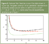
Figure 6
As shown in Billen et al.,12 such a size-independent kinetic plot can be obtained by plotting the separation impedance E13 (originally established by Golay), versus the ratio of N/Nopt. As shown in Equation 3 and Figure 2, it is straightforward to calculate the separation impedance for each data point of the measured Van Deemter-curve:

Equation 3 shows that the vertical difference between two E-curves is still equal to the difference in required analysis time. Because Nopt can be directly assessed from a plot of t 0 /N2 versus N, it is also quite straightforward to calculate the value of N/Nopt for each velocity entry in the spreadsheet table.
Without going into the details, it can be shown12 that a plot of E 0 versus Nopt/N depends only on the dimensionless variables h, ν and φ. A reduced kinetic plot can, therefore, be used for similar purposes as a reduced Van Deemter plot. Packings with the same packing quality and the same retention factor but a different size will yield coinciding curves. And if the curves do not coincide, the column yielding the lower curve can be considered to be better packed. The reduced kinetic plot, however, has two important advantages over the reduced Van Deemter plot. The first one is that it also incorporates the column permeability information and, hence, reflects the quality of the trade-off that is made between column permeability and column efficiency. The second one is that it can be established without having to define or measure a reference diameter, or without having to know the mobile phase diffusivity, thereby providing a way to circumvent the problems mentioned in the Reduced Plate Height section.
Turning now to the two supports considered in the previous figures, the reduced kinetic plot in Figure 7 shows that the slightly larger permeability of the C18-column apparently compensates for its slightly steeper C-term and higher Hmin, as can be witnessed from the fact that both supports have a nearly perfectly overlapping reduced kinetic plot curve. This overlap allows us to conclude that both considered systems display the same intrinsic kinetic quality. Hence, the earlier question that was posed when considering the original plate height and permeability data in Figure 1(a), (i.e., which support performs best or is to be preferred?) can now be unambiguously answered as follows: both support types have the same intrinsic kinetic quality, but they reach their optimal kinetic performance at different values of required N [cf. Figure 3(d)]. However, given the fact that both curves are relatively remote from the best possible packed column line (the green curve in Figure 7), it should also be concluded that, although the two supports perform equally well, they perform relatively poorly.
Comparison of Modern HPLC Supports and Methods
The data shown in Figure 7 have been obtained on several commercial packed columns filled with particles with different size (each curve is the average of two tested columns). The data are represented as a plot of the total analysis time (tR) versus the isocratic peak capacity. The columns were also tested at two different temperatures (30 °C and 80 °C). During these experiments, it was observed that the two tested 3.5 μm columns performed, in relative terms, less well at 80 °C (most probably by coincidence) than the sub-2 μm particles and the 5 μm particles. This behaviour can be observed by comparing the data in Figure 8(a) and (b), showing that the 3.5 μm particles are to be preferred over a much broader range of N-values at 30 °C than at 80 °C.
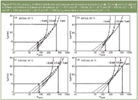
Figure 7
The following main conclusions can be drawn from the kinetic plot curves shown in Figure 8. Provided every support is used in a column with an adapted length, the advantage of an increased temperature is relatively small [compare Figure 8(a) and (b)]. This conclusion might very well be biased by the unexpectedly poor performance of the 3.5 μm particles at the elevated temperature, but for the columns currently studied, the conclusion clearly holds. Larger gains in peak capacity can be obtained by switching to higher pressures [compare Figure 8(a) and (c)], although the gain is certainly not dramatic, and perhaps not worth the additional investment. Comparing Figures 8(a)–(c) with 8(b)–(d) also shows that the advantage of small particles diminishes if columns are run at elevated temperatures. Another conclusion that can be drawn from Figure 8, is that sub-2 μm particles only have an advantage for very short separations, lasting less than 10 s (40 s if a 1000 bar pressure is available).
All these conclusions can be made at a glance, while they would have been nearly impossible to make if the same data would have been plotted in the Van Deemter-curve format.
Establishing a Reliable Kinetic Plot — Practical Considerations
Equations 1 and 2 are based on the t0-marker velocity (u0), because analysts are always most interested in a prediction of the total analysis time, which is most conveniently determined as the product of the t0-time and the (1 + k')-factor. Given that significant differences between the elution time of different t0-markers can be observed, one should preferably always test different t0-markers to find out which gives the most reliable value. Once a good t0-marker is found, it is also important to correct the obtained t0-value for the extra-column volume. This is traditionally done by removing the column and replacing it by a zero dead-volume connection piece to obtain the system dead-time tsys, which can then be used to calculate the t0-time of the column only. The observed variances should also be corrected for the extra-column band broadening, for a kinetic plot can only be established correctly if the plate height values are either corrected for the extra-column band broadening or were not influenced by it. The extra-column band broadening correction can be performed using the following expression:

Ideally, the variances should be calculated using the method of statistical moments because this method automatically and properly accounts for any asymmetry in the peaks. Using the method of moments, columns leading to strongly tailing peaks can then be properly penalized for this. Determining the plate heights using the peak width at half height, however, is easier and less prone to measurement errors, but might in the case of asymmetrical peaks lead to significant errors.
It also goes without saying that the data used to establish the kinetic plot should be obtained with a component that is relevant for the application one has in mind. If desired, kinetic plot curves obtained for a mixture of different components can be combined in one single average curve.14 It is also possible to directly incorporate the limitations (flow-rate limitation, detector sampling rate limitation) of the instrument15 in the kinetic plot curves, but in this case the mathematics are more complex.
Acknowledgement
I would like to thank Deirdre Cabooter for her critical help in the preparation of the manuscript.
Gert Desmet is a full professor in biochemcial and chemical engineering at the Vrije Universiteit Brussel, Brussels, Belgium. His research focuses on the miniaturization of separation methods and on the investigation of flow and mass transfer effects in chromatographic systems.
References
1. G. Rozing, LCGC N. Am., special issue on "Recent Developments in LC Column Technology", ibid (2008).
2. G. Desmet, D. Clicq and P. Gzil, Anal. Chem., 77, 4058–4070 (2005).
3. J.H. Knox and M.J. Saleem, Chromatogr. Sci., 7, 614–622 (1969).
4. J. C. Giddings, Anal. Chem., 37, 60–63 (1965).
5. G. Guiochon, Anal. Chem., 53, 1318–1325 (1981).
6. H.J. Poppe, Chromatogr. A, 778, 3–21 (1997).
7. I. Halász, R. Endele and J. Asshauer, J. Chromatogr., 112, 37–60 (1975).
8. J. H. Knox, Ann. Rev. Phys. Chem., 24, 29–49 (1973).
9. J.C. Giddings, Dynamics of Chromatography – Part I (Marcel Dekker, New York, 1965), pp. 56–60.
10. U.D. Neue, in HPLC Columns: Theory, Technology, and Practice (John Wiley & Sons, New York, 1997), pp. 81–86.
11. D. Cabooter et al., J. Chromatogr. A, 1178, 108–117 (2008).
12. J. Billen et al., J. Chromatogr. A, 1161, 224–233 (2007).
13. P.A., Bristow, J.H. Knox., Chromatographia, 10, 279–289 (1977).
14. D. Cabooter et al., J. Chromatogr. A, 1147, 183–191 (2007).
15. G. Desmet, Anal Chem., 78, 2150–2162 (2006).
Study Explores Thin-Film Extraction of Biogenic Amines via HPLC-MS/MS
March 27th 2025Scientists from Tabriz University and the University of Tabriz explored cellulose acetate-UiO-66-COOH as an affordable coating sorbent for thin film extraction of biogenic amines from cheese and alcohol-free beverages using HPLC-MS/MS.
New Study Investigates Optimizing Extra-Column Band Broadening in Micro-flow Capillary LC
March 12th 2025Shimadzu Corporation and Vrije Universiteit Brussel researchers recently investigated how extra-column band broadening (ECBB) can be optimized in micro-flow capillary liquid chromatography.


