The LCGC Blog: Why Every Good Analytical Chemist Also Needs to Be a Statistician

June 15, 2015

Article

Once you have mastered the terminology and symbology the actual mathematics for the models and approaches used at the level which is useful to practicing analytical chemists is really very straightforward indeed.

I’ve just been greatly assisted by a Thirteenth Century mathematician from Pisa. But more on that in a moment.

I presume most of you working in the pharmaceutical industry will, by now, have seen the updated Food and Drug Administration (FDA)

Guidance for Industry Analytical Procedures and Methods Validation for Drugs and Biologics

This replaces the Draught Guidance of 1987 (updated in 2000) which remained for its whole operational lifetime a draught document and was never finalized (!) Let’s hope that this one makes it onto the statute – so to speak.

While there are several changes from the 2000 document, section VII. STATISTICAL ANALYSIS AND MODELS, is among the most significant. The text describes the use of statistical analysis of validation data to evaluate the method and validation characteristics against pre-defined criteria. It also describes the use of multi-variate models in analytical methods and the testing of these models using an appropriate number of samples and deliberately varied parameters. Those of you with any sense of statistical analysis will realize this is more than cursory nod to the use of so-called "Quality by Design" statistical approaches.

This, in a roundabout way, brings me to my point. You either like statistics (and statistical analysis) and get it, or you struggle with it. I’m pleased to say that I’ve always "got it" and actually enjoy statistical analysis and modelling very much. Once you have mastered the terminology and symbology the actual mathematics for the models and approaches used at the level which is useful to practicing analytical chemists is really very straightforward indeed.

A quick example. The following formula looks pretty daunting:

In fact it’s the formula for calculating the standard deviation of a sample population (s) (only the standard deviation of a whole population is called σ, by the way), which can be done very simply on a scientific calculator or using Microsoft Excel ™. You can of course work it out long hand (using the calculator for the simple mathematical operations) - like for the following example data which represents six replicate injections of a standard used to measure autosampler reproducibility;

(Result)

101.2
100.5
99.7
99.2
100.3
100.1

1.03
0.33
-0.47
-0.97
0.13
-0.07

1.0609
0.1089
0.2209
0.9409
0.0169
0.0049

(mean)
Sum of all values / 6

100.17

Total

2.3534

(I checked the value in Excel and it gives the same answer!)

If you work in analytical science and are in any way involved with method validation and robustness testing or analytical method optimization, you will be using statistical approaches and, since the introduction of the new FDA Method Validation guidance mentioned above, the use of statistics will only be increasing in the future.

However, even if you "don’t get it" or "aren’t a fan" or simply haven’t tried any of the more in-depth approaches, you are missing out on a wonderful world that can help you enormously, even at the level which is possible with common tools such as Microsoft Excel ™.

As well as the usual statistical descriptors which we commonly use (mean, standard deviation, relative standard deviation, co-efficient of variation) there is a world of useful tools, which you really don’t need to have a "statistics" department to make use of, and which can be easily done in Microsoft Excel ™.

Of course we have the usual methods of linear regression to test trueness of fit of a calibration function (most of us use the Product-Moment correlation co-efficient (r) to measure this), which should always be accompanied by an estimation of the error (standard deviation) in the slope and intercept of the fitted line using residuals, in order that we can give state the likely error associated with any value interpolated from the fitted curve. The t-test (for comparing mean values) can be used to test for systemic error in a chromatographic method (is the mean of our analytical results significantly different from the level at which the sample was spiked?) or to compare two means (are the results between two analysts validating a chromatographic method significantly different?).

A paired t-test can tell us if the results of our new improved separation (after transfer to a short, narrow i.d. GC column at higher carrier gas linear velocity for example), gives statistically significantly different results from the original method, or is it, as we hope, just significantly faster. As well as testing all of the results above to see if the results are different, we can use an F-test to see if the methods differ in precision by testing the standard deviations of the results. We can use the Grubbs or Dixons tests to identify outliers in our data, and we can use simple analysis of variance (ANOVA) to measure within day and between day precision during method validation. All of these tests can be achieved using the basic statistical functions within Microsoft Excel ™.

If one wishes to utilize some of the most useful aspects of statistical experimental design and optimization, then one would need to use a simple statistical tool such as Minitab ™. Many of you reading this will think I’ve strayed into the land of the statistician – but not so. This program is very easy to use, and with only a rudimentary understanding of the principles, can help us to improve our analytical practice enormously.

For example, it is very straightforward to plan, implement, and analyse Fractional Factorial designs which allow us to investigate the dominant variables within a method and help to control them more effectively. We can use the same methods for identifying interactions between variables in our methods and control or eliminate them. It is very easy to plan a fractional factorial design such as the Plackett-Burman, in order to significantly reduce the number of experiments required to validate an analytical method for Robustness. We can also use full factorial methods to optimise an analytical method in significantly fewer experiments using the tools available within Minitab™. Oh – and for those you who would rather leave all of this math to your "statistics department" – two things. First – what if you aren’t lucky enough to have a statistics depertment? Second – the statisticians will come to ask you which variables you would like to test and what levels (ranges) you would like to test them over, and whether there is likely to be any interaction between variables. So you can’t just wash your hands and say it’s "not your thing," as only someone with good analytical experience and a knowledge of the method under investigation can answer these questions meaningfully.

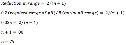
That brings me back to my Thirteenth Century mathematician – Fibonacci. I wanted to optimize the pH of a separation to achieve the best resolution between a critical pair of analytes whose logD values differed. I had no idea what the logD values were however, so the actual range for the experiments was 8 pH units (pH2 – pH10, the working range for good stability of the silica support within the HPLC column) and I wanted to specify the pH to within 0.2 pH units, as I know the separation is sensitive to pH changes and therefore wanted to ensure the correct robustness. If I make sequential measurements to locate the optimum pH based on the previous two results, I can calculate the number of experiments required using the formula;

I didn’t fancy doing 79 experiments! So I turned to an old friend – The Fibonacci series (shown below), which can be used to significantly reduce the number of required experiments in an optimisation such as this, and in which each number represents the sum of the previous two.

F10

F11

In order to achieve a 40 fold reduction in range for our optimum pH (8/0.2), then I take the first Fibonacci number above 40 (F10,55), and the subscript tells me I will need 10 experiments. Further, the series tells me how to carry out the experiments. I take F10 and divide it into the number TWO BELOW in the series (F8) and the resulting number gives me the INTERVAL for my first experiments.

(the number 8 here represents the original pH range)

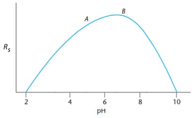
Therefore my first experiments are at pH 2+3.1 and pH10 – 3.1 or pH5.1 and pH6.9 respectively.

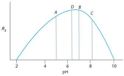
Experiment B produces the highest response and therefore the maximum must be between A and 10. A new measurement (C) is made so that A – C is the same distance as B – 10 (i.e. 8.2) and a measurement (D) is made such that the A – D and B-C distances are equal (B – C is 1.3) therefore D is at 6.4.

Further measurements are made until the distance between the maxima of two subsequent measurements <0.2 pH units. In this case we found a suitable optimum with exactly 10 experiments.

Of course – using predictive modeling software (several are available for chromatographers), I may have been able to achieve this in much fewer experiments (intuitively I think six experiments would have been enough), and it is possible to optimize several variables simultaneously. However 10 experiments for this simple univariate optimization is certainly better than 79!

So – there endeth the lesson on why you should grow to love statistics. These approaches and methods can help us to more accurately specify our results, give estimations of error, plan experiments, validate methods, and optimize our separations. We simply can’t do first rate analytical work without the use of statistics and statistical models, and if this piece has served to stir your interest, I cannot recommend the following text by James and Jane Miller highly enough – enjoy!

Statistics and Chemometrics for Analytical Chemistry, J.C. Miller and J.N. Miller, Sixth edition 2010, Pearson Education Limited, ISBN: 978-0-273-73042-2

For more information, contact either Bev (bev@crawfordscientific.com or Colin (colin@crawfordscientific.com). For more tutorials on LC, GC, or MS, or to try a free LC or GC troubleshooting took, please visit www.chromacademy.com