The LCGC Blog: A Weighty Problem with Calibration

Chromatographic methods often require that the analyte response is calibrated (and validated) over a wide concentration range when the analyte concentration in the sample is either unknown or is expected to vary widely. Bioanalysis, environmental, and clinical applications are just a few examples of where this may be the case.

No matter how linear the detector response, the need to cover wide concentration ranges can present us with problems with homoscedasticity or the assumption that variance is equal across the whole calibration range, independent of analyte concentration. In fact the use of fitted regression models using least-squares estimators requires this to be the case in order to give unbiased estimates of the concentration of our unknowns.

This problem typically presents itself as poor accuracy (bias) when determining smaller analyte concentrations as the higher concentration data tends to have larger variance which unfairly influences (weights) the regression model.

Once problems with homoscedasticity of the data have been identified and confirmed, it is often relatively straightforward to overcome the issues using weighted least squares linear regression models, however there tends to be a reluctance or nervousness in this approach. It’s almost as though unless we use unweighted linear regression models. We fear challenge to an “atypical” approach, and the use of non-linear or weighted models will draw extra scrutiny that will be very difficult to justify. We are somehow trying to use mathematics to overcome issues with our methods. I’ve seen people redevelop methods in order to try and overcome these issues, wasting a lot of time and effort.

We simply need to accept that some analytical methods do not produce a linear response and, as we will examine here, that the data may not have equal variance which is independent of analyte concentration. Also, under these circumstances the use of weighted regression models is required. I believe the main “fear” in the use of these “less conventional models” is the burden of justifying the approach, and hopefully I can demonstrate with a relevant example that, for the use of weighted regression at least, the justification can be relatively straightforward.

So here are the data for the calibration curve under investigation:

The unweighted least squares regression model output is:

Slope (a) = 6.4916

Intercept (b) = -0.3461

Coefficient of determination, r² = 0.9980

Figure 1: Unweighted linear regression model for the data in Table 1

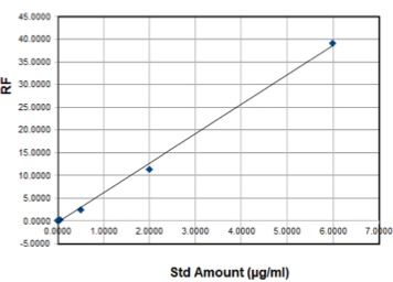
On the face of it, the regression co-efficient (r2) seems to indicate linearity and the data seems to fit the regression model (trend line in Figure 1).

However, a simple “eyeball” of the regression results does not allow us to properly investigate the validity of the model.

Due to some prior knowledge of the application and likely sample concentration ranges, the following data was produced in order to the test the regression model.

The % Relative Error allows a quantitative estimate of the error in each determination and is calculated as follows:

%RE = ((Calculated Concentration - Nominal Concentration) / Nominal Concentration) x 100

Table II: Validation data for regression model

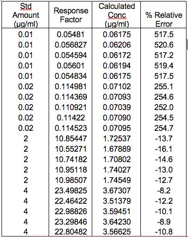
It’s important to state here that the higher the number of determinations at each calibration level, the higher the confidence we can have into the results of the investigation (6 independent determinations at each concentration level is typical) and that having data at the upper and lower end of the range will also help to investigate the model more thoroughly.

The results for the standard solutions would be unusable with huge associated error. This data is typical of the situation in which the larger variance of standards at higher concentrations drastically skews the results for the determinations at lower concentration and we suspect heteroscedasticity within the data. There are two checks that might be made in this case:

• Construct a regression model from the data in Table II and examine the residuals plot

• Carry out an F-test using the highest and lowest data points in the validation data and test to see if there is a significant difference in the variances of the two populations (for example, the data for the highest and lowest calibration standards)

The residuals plot from the regression analysis of the data is shown in Figure 2 alongside of the F Test results (Table III). All of the data was generated in Microsoft Excel using the Data Analysis Toolpack Add-In.

Figure 2: Residual plot for the validation data in Table II

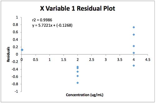
Table III: F-Test result from the 0.01 and 4 ug/mL Standard data from Table II

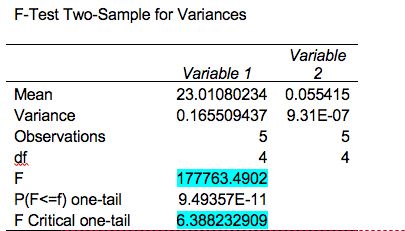
As can be seen from Figure 2, the residuals form a “fan” shape from lower to higher concentrations and this is generally typical of heteroscedastic data in analytical calibration models, visually demonstrating the increasing variance with analyte concentration.

In order to further verify heteroscedasticity an F-test was performed using the variance of the higher concentration data (s₂) versus the lower concentration data (s₁) according to the following equation:

From the data shown in Table III, it is clear that the calculated F value (177763.4902) far exceeds the critical value for F (one-tail test) (6.388232909), and therefore there is a strong indication that the variances of these two populations are not equal.

This evidence of heteroscedasticity is justification for the consideration of a weighted least squares calibration model.

The key question is, which weighting to apply and it is here that users often become discouraged due to a lack of a definitive methodology to assess the effects of the various weightings. One further discouraging factor is that Microsoft Excel does not offer a function for weighted regression – however several are available online with my favourite being found at the following link:

http://terpconnect.umd.edu/~toh/models/CalibrationCurve.html

(select the weighted linear regression spreadsheet and download it)

Note also that your data system may be capable of automatically calculating the weighted regression which will save a lot of manual data processing.

One helpful method to assess the performance of each weighting method is to measure the Σ%RE for each of the validation data points using the various weighting schemes and assess this number alongside the residual plot for each weighting. The best model will usually be that which produces the lowest Σ%%RE value alongside a residual plot which shows a much more even distribution of variances across all of the concentration levels within the range. Table IV shows this data for the unweighted and 1/x weighted data and Table V shows the results of the assessment of all different weighting methods:

Table 4:

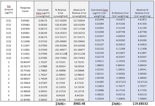
Table V: Results from the assessment of various calibration models using the validation data of Table II

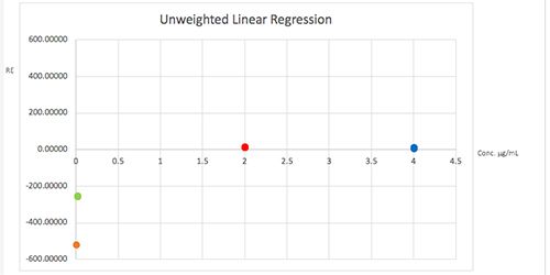
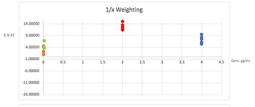
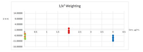
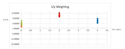
Figure 4: Plots of total error in the determination of the validation data of Table II using various weighted least squares regression models, used to assess the distribution of error across the range of concentrations

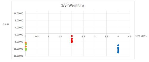
From Table V it would seem that the 1/x² weighting produces the lowest S%RE, and Figure 4 helps to highlight the problem with the unweighted data and indicates a more even distribution of variance across of the calibration concentrations. I believe that this is strong evidence to justify the use of the 1/x² weighted least squares regression model for this determination.

It should be noted that while in this example the error plots do not greatly differ on visual examination, in some examples they can be vital in helping to choose the correct model and justifying the approach.

Of course this is only one facet of the investigation of the calibration model statistics, and one might argue that the regression data may indicate that non-linear effects are observed (the U shape of the residuals data in Figure 2). Next time we will investigate the goodness of fit for linear versus quadratic calibration curves to help define the most appropriate calibration model.

Tony Taylor is the technical director of Crawford Scientific and ChromAcademy. He comes from a pharmaceutical background and has many years research and development experience in small molecule analysis and bioanalysis using LC, GC, and hyphenated MS techniques. Taylor is actively involved in method development within the analytical services laboratory at Crawford Scientific and continues to research in LC-MS and GC-MS methods for structural characterization. As the technical director of the CHROMacademy, Taylor has spent the past 12 years as a trainer and developing online education materials in analytical chemistry techniques.